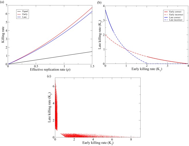
FIG 3.

Killing rates predicted by equation 17. (a) The red line depicts K₁ for K₂ = 0 as a function of ρ, the blue line K₂ for K₁ = 0 (see equations 18a and b, respectively), and the black line is just the line K = K₁ = K₂ = ρ. (b) K₂ is depicted as a function of K₁ for ρ = 1, using equation 17b for the early killing parameters, d₁ = γ = d₂ = 1 (in red), and for the late killing parameters, d₁ = 0.1, γ = 1, and d₂ = 2 day⁻¹ (in blue). Note that we indeed predict that the lines cross at K₁ = K₂ = ρ = 1. The lines are solid when 0.5 < δ < 1.5 and dashed otherwise. (c) We make small steps through the parameter space for 0.01 ≤ d₁, d₂ ≤ 5, and 0.5 ≤ ρ ≤ 1, drawing a random value for either K₁ or K₂ from a uniform distribution, 0 < K₁, K₂ < 10, and use equation 17a or b to compute the other killing rate. This analysis is performed for γ = 1, and we increase the parameters by 10% when we step through the parameter space. Here, we are more strict and only accept solutions when 0.75 < δ < 1.25 (in the presence and absence of CTL).