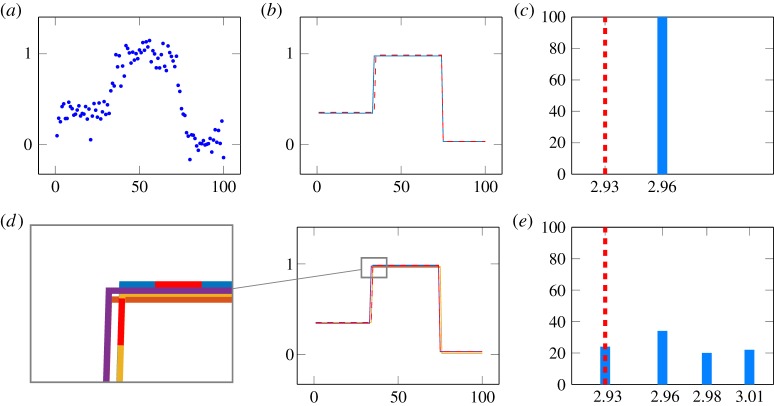
Figure 4.

Influence of the starting point on the result of the iterative Potts algorithm (γ=1): for small random perturbations of the starting point, we end up the same local minimizer for all 100 realizations. The result is near to the global minimizer which is displayed as dashed line (b). For large random perturbations, we obtain four different nearby results (d). The histogram shows their frequency where the abscissa displays their functional values (e). The dashed line indicates the global optimum which could be computed for this particularly simple example by brute force. (a) Blurred and noisy signal. (b) Result with perturbed starting point (τ=0.01). (c) Histogram of the local minimizers (τ=0.01). (d) Results with perturbed starting point (τ=0.5). (e) Histogram of the local minimizers (τ=0.5). (Online version in colour.)