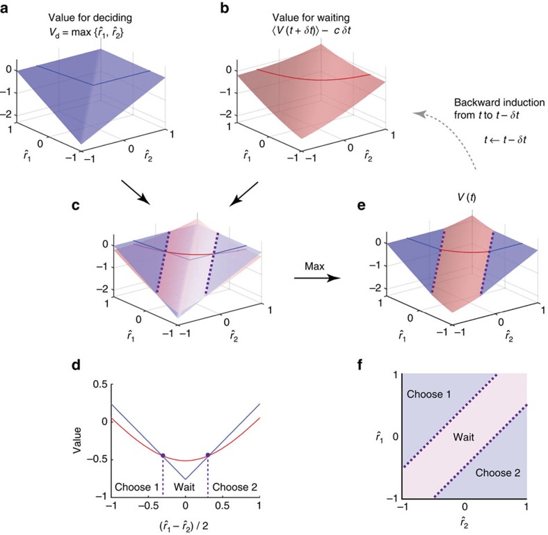
Figure 3. Finding the decision boundaries in value-based decision.

(a) The expected values of choosing either option are defined as a two-dimensional function (surface), , of a pair of reward estimates, , at time t. The dark coloured line shows the section at . (b) Similarly, the value surface for ‘waiting' (that is, the expected value after observing new evidence for a short period δt, subtracted cost for waiting cδt) is defined as a function of . Note that, around the diagonal, , the value for waiting is smoother than that for choosing due to the uncertainty about future evidence. (c,d) The value surfaces for choosing and waiting superimposed, and their sections at . The decision boundaries (dotted lines) are determined by points in the space of reward estimates in which the value for ‘deciding' (blue) equals that for waiting (red). In the region where waiting has a higher value than choosing either option (blue below red curve/surface), the decision maker postpones the decision to accumulate more evidence; otherwise, she chooses the option that is expected to give the higher reward. Because the relationship between the two value surfaces is translational symmetric in terms of mean reward , their intersections are parallel and do not depend on this mean reward. (e) The expected value V(t) is given by the maximum of the values for choosing and waiting. This surface determines the value for waiting (b) at the next-earlier time step, t−δt. (f) Decision boundaries and associated choices shown in the two-dimensional representation. Note that the two boundaries are always parallel to the diagonal, . This is because the both value functions (for deciding and for waiting) are linearly increasing with slope one in lines parallel to the diagonal (a,b). For the value for deciding, for example, below the diagonal we have , such that , and therefore , where C is an arbitrary scalar. The value for waiting can be shown to have the same property.