Search performance is better predicted by tileability than presence of a unique basic feature

Abstract

Traditional models of visual search such as feature integration theory (FIT; Treisman & Gelade, 1980), have suggested that a key factor determining task difficulty consists of whether or not the search target contains a “basic feature” not found in the other display items (distractors). Here we discriminate between such traditional models and our recent texture tiling model (TTM) of search (Rosenholtz, Huang, Raj, Balas, & Ilie, 2012b), by designing new experiments that directly pit these models against each other. Doing so is nontrivial, for two reasons. First, the visual representation in TTM is fully specified, and makes clear testable predictions, but its complexity makes getting intuitions difficult. Here we elucidate a rule of thumb for TTM, which enables us to easily design new and interesting search experiments. FIT, on the other hand, is somewhat ill-defined and hard to pin down. To get around this, rather than designing totally new search experiments, we start with five classic experiments that FIT already claims to explain: T among Ls, 2 among 5s, Q among Os, O among Qs, and an orientation/luminance-contrast conjunction search. We find that fairly subtle changes in these search tasks lead to significant changes in performance, in a direction predicted by TTM, providing definitive evidence in favor of the texture tiling model as opposed to traditional views of search.

What makes search easy or hard?

What determines the difficulty of searching for a target such as a friend in a crowd or a lesion in a medical image? Visual search has fascinated generations of researchers, both for its real practical importance, and as a window into visual processing. Fully understanding search requires studying both stimulus-specific factors, such as how easy it is to discriminate the target from other parts of the display, as well as higher-level factors such as expertise, priors on the location of the target, and decision-making (Oliva, Torralba, Castelhano, & Henderson, 2003; Wolfe, Butcher, Lee, & Hyle, 2003; Oliva, Wolfe, & Arsenio, 2004; Wolfe, Horowitz, & Kenner, 2005). To isolate stimulus-specific factors, search experiments often use simple displays consisting of a search target and a number of distractors, where the target appears with equal probability in one of the possible item locations. Typically, researchers plot the time to correctly respond whether or not a target is present (the reaction time, or RT) as a function of the number of items in the display (the set size). The slope of this function provides a common measure of search difficulty known as the search efficiency—the number of items processed per unit time—allowing the categorization of search tasks into efficient and inefficient search (Wolfe, 1994).

According to FIT, search is easy if and only if the target contains a basic feature not found in the rest of the display (Figure 1A). This suggests the extremely attractive idea that a simple behavioral experiment might inform us in a straightforward way about basic feature detectors early in vision. These basic features (e.g., orientation, motion, or color), are presumed to be available preattentively and in parallel across the visual field, leading to rapid search. If the target differs from the distractors only in a conjunction (e.g., red and vertical) or configuration of features (red to the left of green), then FIT predicts difficult search, because the observer will have to serially attend to each item in order to bind the features and identify the target (Treisman & Gelade, 1980). FIT has explained a number of classic search phenomena, though a number of researchers have also pointed out issues both regarding FIT's ability to predict search results, and regarding the notion that only maps of basic features are available in preattentive vision. (e.g., Carrasco, Evert, Chang, & Katz, 1995; Carrasco, McLean, Katz, & Frieder, 1998; Carrasco & Yeshurun, 1998; Vlaskamp, Over, & Hooge, 2005; Wertheim, Hooge, Krikke, & Johnson, 2006; Reddy & VanRullen, 2007; Rosenholtz et al., 2012a; Hulleman & Olivers, 2015).

Figure 1.

Comparison of two visual search models. (A) Rule of thumb for the traditional feature integration theory (FIT). FIT is a word-model that operates on descriptions of the target and distractor items. As such, it allows for easy intuitions, enabling design of new and interesting experiments. However, it is inherently under-specified without a complete description of basic features. (B) The texture tiling model (TTM). TTM is an image-computable model which takes as input image patches from the search display. Its features—a rich set of local image statistics—are fully specified. However, due to this complex set of features, TTM does not as easily lend itself to intuitions, making design of new experiments more difficult. Here we work to develop a TTM rule of thumb, to facilitate understanding of the model and intuitions about its predictions.

We have recently shown that an alternative model, TTM, also explains a number of classic results (Rosenholtz et al., 2012b). TTM puts the blame for many difficult search tasks not on the limits of preattentive vision, but rather on the limits of peripheral vision (Rosenholtz et al., 2012b).

Peripheral vision has considerable loss of information relative to the fovea. Its well-known reduction in visual acuity has a modest effect compared to visual crowding. In crowding, observers can have difficulty identifying a peripheral target when it is flanked by other display items, even when those items lie quite far from the target. Behavioral work suggests that the critical target-flanker spacing is approximately 0.4 to 0.5 times the eccentricity (the distance to the center of fixation) of the target, for a fairly wide range of stimuli (Bouma, 1970; Pelli, Palomares, & Majaj, 2004).

The critical spacing of crowding suggests that peripheral vision processes sizable patches. In an often-cluttered search display, such patches likely contain multiple elements. For a given fixation, one patch may contain only distractors. Another may contain distractors plus the target. If the observer can easily tell apart a peripheral target-present patch from a target-absent patch (Figure 1B), search should be easy. If peripheral information is insufficient for the discrimination of the two types of patches, search will be difficult because the observer will need to move their eyes to regain the lost information. The key is to understand the information available in peripheral vision.

TTM hypothesizes that peripheral vision “compresses” its inputs, by representing them in terms of a rich set of local image statistics. In particular, we use the statistics identified by Portilla and Simoncelli (2000) for the purposes of capturing the appearance of visual texture. Portilla and Simoncelli (2000) first process the input with a multiscale, multiorientation steerable pyramid. Then, in addition to computing statistics such as the marginal distribution of luminance and the luminance autocorrelation, they compute correlations of the magnitude of responses of that pyramid across differences in orientation, neighboring positions, and scale, and phase correlation across scale. This is simpler than it may sound; computing a given second-order correlation merely requires taking responses of a pair of subbands (a subband is the output of the pyramid for a given scale and orientation), point-wise multiplying them, and taking the average over the specified region. These statistics are sufficient to capture information about the distribution of luminances and orientations present in a patch, as well as the sharpness of edges. The statistics signal the existence of junctions—the representation does not consist merely of a collection of oriented lines. The various correlations also encode a sort of “proto-grouping”; they capture sufficient information to preserve regions of similar features as well as extended contours.

The original image can be perfectly reconstructed from the full multiscale pyramid. However, the summary statistics described above cannot unambiguously specify the original stimulus. The summary statistics involve averaging or pooling over space, which loses information. We hypothesize that the resulting ambiguity about the contents of the stimulus leads to visual crowding (Korte, 1923; Bouma, 1970; Lettvin, 1976).

To validate TTM, we have tested its ability to predict performance on a range of peripheral tasks. We have generated and tested predictions in the following way. We first use the Portilla and Simoncelli (2000) texture analysis/synthesis technique to synthesize, for a given local image patch, other patches with approximately the same image statistics.¹ We call these syntheses “mongrels.” They look like jumbled versions of the original patch. Mongrels allow us to visualize the information encoded by the model statistics. A number of unique patches have the same statistics as the original; in practice, we generate around 10 mongrels per stimulus patch. We then have observers perform tasks with these mongrels. In the case of visual search, for example, observers attempt to distinguish target-absent from target-present patches. If the mongrel discrimination is difficult, TTM predicts peripheral discriminability will be difficult, as will search.

Other means of testing the model are possible. Freeman and Simoncelli (2011) demonstrated that a full-field version of this encoding can produce visual metamers for a fixating observer. Alexander et al. (2014) showed that observers performing a search task made different saccades to an array of teddy bears than they made to an array of teddy bear mongrels (synthesized using only local summary statistics). This suggests that peripheral vision has access to additional shape features, either through additional summary statistics or through interactions of multiple overlapping pooling regions. We have preferred tests of task performance; they degrade gracefully if the peripheral encoding model is not perfectly correct, which is almost certainly the case here.

TTM has done well so far. We have shown that it explains not only search performance, including four of the tasks discussed here (Rosenholtz et al., 2012b), but also performance identifying a peripheral symbol (Balas et al., 2009; Keshvari & Rosenholtz, 2016), and getting the gist of a scene (Rosenholtz et al., 2012a; Ehinger & Rosenholtz, 2016). It seems that the model does well at capturing information available and lost by the encoding in peripheral vision.

The need both to synthesize images with the same statistics and to have observers perform tasks with those syntheses (in our methodology as well as that of Freeman & Simoncelli, 2011, and Alexander et al., 2014) has perhaps discouraged other researchers from testing TTM. Here, one of our goals is to uncover a more intuitive rule of thumb for TTM, to enable more widespread testing.

Our main goal, however, concerns discriminating between models of visual search. Both FIT and TTM can predict the results of a number of classic search experiments. Here we seek a tie-breaker: new search experiments for which the models make different predictions.

A rule of thumb for the texture tiling model

FIT's rule of thumb (Figure 1A) enables easy intuitions, which has led to decades' worth of interesting experiments. To design experiments to compare FIT and TTM, we here develop a rule of thumb for the latter by examining mongrels from five classic search tasks (Figure 2). In this paper, as in our previous syntheses for single pooling regions (Balas et al., 2009; Rosenholtz et al., 2012a; Rosenholtz et al., 2012b; Zhang, Huang, Yigit-Elliott, & Rosenholtz, 2015), we generate mongrels using Portilla and Simoncelli's (2000) texture analysis/synthesis routine, with parameters (number of scales = 4, number of orientations = 4, neighborhood size = 9).

Figure 2.

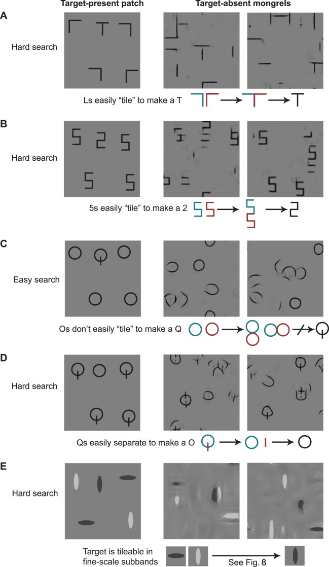
Why does TTM predict that classic search conditions are easy or hard? For five classic search tasks (target-present patch in column 1), we synthesized two images having approximately the same summary statistics as a target-absent patch. We call these synthesized images mongrels. Mongrels visualize the information encoded by the model and ambiguities due to lost information. For the difficult search tasks, the mongrels show target-like figures even though the original patch contained no target (respectively, a T, 2, O, and black vertical). Therefore, TTM predicts that peripheral vision will have difficulty distinguishing target-present from target-absent patches, leading to difficult search. What causes the target-like figures? Diagrams below the first four conditions show the hypothesized origin. We discuss conjunction search later (see Figure 8).

Clearly, representation in terms of image statistics leads to an ambiguity between the original stimulus and jumbled versions of that stimulus. If we compare the target-absent mongrels of easy Q among O search with those of the four more difficult tasks, we can see an interesting difference. The mongrels of O-only patches contain no Q-like items (Figure 2C), whereas for all other conditions, the mongrels of target-absent patches can contain target-like items. In the difficult search tasks, the image statistics are ambiguous in a way detrimental to efficiently finding the target. Where do these target-like items come from? For the T among L search (Figure 2A), the T-like items in target-absent mongrels may arise from lining up and piecing together two differently oriented Ls, tiling them together. Similarly, 2-like items seem to tile from a pair of 5s (Figure 2B). Note that these illusory targets need not appear in every mongrel for the model to predict difficulty discriminating target-absent from target-present patches, leading to difficult search.

In the target-absent patches of easy Q among O search, Os can't easily tile to form a Q in the same way (Figure 2C). This means that according to TTM, peripheral target-absent patches are less likely to be confused with target-present patches, making search for Q among O easier.

Difficult O among Q search shows somewhat the opposite effect. In target-absent mongrels, Qs exhibit the dual of tiling: they disperse, leaving isolated vertical bars and O-like forms. This ambiguity may mislead the observer about the presence of a peripheral target O (Figure 2D). As the conjunction search story is more complicated, we discuss it later after further developing the basic intuitions (see Figure 8).

Figure 8.

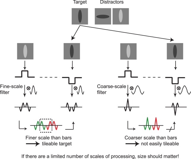
Tileability and conjunction search. Shown are 1-D bars, and the result of filtering those bars with fine scale (left) and coarse scale (right) bandpass filters (e.g., with a Gaussian second derivative). The fine-scale filter responses to a distractor light bar can be tiled to form a target dark bar. However, the same is not the case for the coarse-scale filter responses to a light bar. This suggests that thinner bars may lead to fewer illusory conjunctions.

These examples suggest the following rule of thumb: Crowding in peripheral vision leads to ambiguities between an original patch and jumbled versions of that patch. If in that jumbling, distractors can easily tile to produce a target, search is hard; otherwise, search will be easy. In later sections, we will elucidate the meaning of this rule of thumb, and give a better sense of what tiling means as we design variants to classic search tasks. In particular, we will suggest that two portions of a local patch can join or tile if they contain a similar set of local orientations. However, this can only occur if their joining does not change the summary statistics of the patch as a whole. Neighboring portions of a patch can also disperse if grouping between them is weak and if the place where they meet has features similar to other parts of the patch, so that when they disperse, they have somewhere else to go and join. Finally, we will clarify that tiling should really be thought of as happening in subbands rather than in pixel space, and discuss the implications for conjunction search.

Of course, peripheral vision also causes ambiguities in target-present patches. They may also jumble, perhaps eliminating anything like a target, again leading to difficult search. In fact, for classic T among L search we often see no target in mongrels of target-present patches, as well as illusory targets in mongrels of target-absent patches. However, for the classic search conditions under examination, TTM predicts a significant amount of the difficulty lies in representation of target-absent patches. In our experience, it is difficult to construct an interesting search condition with good representation of target-absent patches yet poor representation of target-present patches—interesting in the sense that not all models predict difficult search. If target-absent patches can be well encoded by peripheral vision, often so can target-present patches, so long as the target is sufficiently discriminable from the distractors. As a result, here we focus on representation of target-absent patches.

Tileability suggests interesting modifications to classic search tasks

Fully specifying FIT would require enumerating all of the basic features available preattentively. This makes it difficult to generalize to novel search stimuli, and makes FIT itself somewhat of a moving target. To get around this issue, rather than designing totally new search tasks, we start with five classic search tasks that FIT has previously explained using its accumulated rules of thumb. As we know FIT's explanation for performance on those tasks, if new search tasks use similar-enough stimuli we should be able to generalize FIT's predictions to those tasks.

Specifically, we modified five classic search experiments by making subtle changes to the stimuli. We do so in order to manipulate tileability, while maintaining insofar as possible the presence or absence of commonly accepted basic features. By thus pitting predictions of FIT and TTM against each other, we can definitively compare the two models.

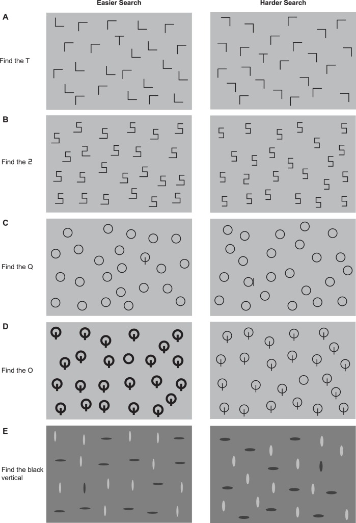
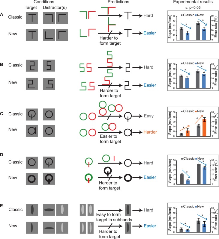
Figure 3 shows examples of the classic and new search tasks. We discuss the rationale for the new search tasks in the following sections. Tileability predicts, for each condition, that these subtle changes to the stimuli will change search performance in a particular way, making it easier in some conditions, and harder in others. Though we focus on the rule of thumb for TTM in this paper, as opposed to our usual methodology for making predictions for TTM (e.g., Zhang et al., 2015), for each condition, we generate several mongrels to check our intuitions derived from the notion of tileability.

Figure 3.

Five classic search tasks and our new modified conditions. Tileability predicts that the conditions on the left are easier than those on the right, a result borne out by our experimental results. (A) Classic condition on the right. The true classic task involved four possible orientations of both T and Ls. (B) New task with longer bottom bar shown on the left. (C) New task, with vertical bar moved, on the right. (D) New task with thicker lines on the left. (E) New task with thinner bars on the left.

In general, FIT-based models do not obviously predict that these manipulations should have any effect. Below we discuss each of the stimulus manipulations, and then present experimental results.

T among L

Traditional search for a T among Ls, where both the T and Ls could appear in any of four 90° rotations, is relatively slow and difficult, requiring 20–30 ms/item for target-present trials (Wolfe, 2001). Wolfe proposed that this search is inefficient because targets and distractors share the same basic features, i.e., Ts and Ls are both composed of a vertical and a horizontal line element (Wolfe, 2001). Recall that target-absent mongrels for this condition suggested that this search task might instead be difficult because two Ls could tile to form an illusory T. Might we make a change to the stimulus that would reduce the probability of tiling to form a T? It would seem a challenge to keep Ls at any orientation from forming a T at any orientation. But what if we limit the target to an upright T? Are some orientations of Ls worse than others for making search for an upright T difficult?

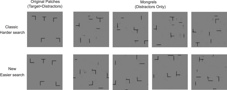
For convenience, we label the four oriented Ls as follows: L₀ represents a normal, upright L; L₉₀, L₁₈₀, L₂₇₀ represent Ls rotated clockwise by the indicated number of degrees. One can place L₁₈₀ (similar to the left half of a T) and L₉₀ (similar to the right half of a T) next to each other to make something like an upright T. The two Ls share many of the orientations and co-occurrences of orientations present in the T, making this a plausible tiling. (Of course, we do not see in the mongrels a T made by literally piecing together two Ls. Such a T would be too large, violating image statistics measured at a coarser scale. Rather, the pieces left over from tiling two Ls into a T appear as additional structures elsewhere in the mongrel.) One can perhaps not so easily tile L₀ and L₉₀ to make an upright T while remaining consistent with the measured statistics. Tileability predicts that search for an upright T among (L₀, L₉₀) will be an easier search than among (L₁₈₀, L₉₀).

However, there is a subtlety to this claim. If we flip L₀, we get L₁₈₀. An image containing only L₀ actually has the same statistics as one containing only L₁₈₀ (this is just a consequence of Fourier theory, plus pooling of statistics; see Zhang et al., 2015). This might suggest that (L₀, L₉₀) could tile to make an upright T just as easily as (L₁₈₀, L₉₀), since L₀ and L₁₈₀ are ambiguous. However, in multi-item displays, coarser scales provide additional information. Neighboring Ls can trigger responses of horizontal and/or vertical filters at a coarser scale, even if the Ls are not perfectly aligned. In an (L₀, L₉₀) patch, it may be difficult to preserve coarser scale statistics if one flips an L₀ to an L₁₈₀ without also flipping the L₉₀ into an L₂₇₀, again making tiling into an upright T unlikely. We have examined a number of mongrels from these two conditions, to confirm these intuitions (see Figure 4 for examples). We compare search for an upright T among (L₁₈₀, L₉₀) to that among the less-likely-to-tile (L₀, L₉₀). For brevity, we refer to the former condition as the “classic” search condition, as it should have a similar tiling issue as classic T among Ls. Note that comparison with the truly classic T among Ls would be an unfair comparison, as that condition has both more possible targets and more heterogeneous distractors. Increasing target uncertainty leads to more difficult search, all else being equal. It is also known that when target–distractor discriminability is low, increasing distractor heterogeneity results in decreased search efficiency (Bergen & Julesz, 1983; Duncan & Humphreys, 1989).

Figure 4.

Mongrels for T among L search, old and new conditions. Note the prevalence of illusory Ts in the mongrels for the classic search (top) as opposed to the new search condition (bottom), as predicted by tileability.

With the same basic features, same target uncertainty, same distractor variability, and the same need for binding of horizontal and vertical bars to distinguish target from distractors, models like FIT should predict that our “classic” and “new” tasks are equivalently difficult. We predict that the new task will be easier, because the distractors cannot as easily tile to make a target.

2 among 5

Classic search models explain the difficulty of search for a 2 among 5s as due to the target and distracters sharing the same basic features—presumably the component horizontal and vertical bars—and differing only in the configuration of those basic features. At a coarse scale, the target and distractors actually do have a different, although weak, dominant orientation, which one can see by greatly blurring the items. (A 5 has energy oriented at about 20° to the left, and a 2, at about 20° to the right.) However, this difference apparently does not suffice to support efficient search.

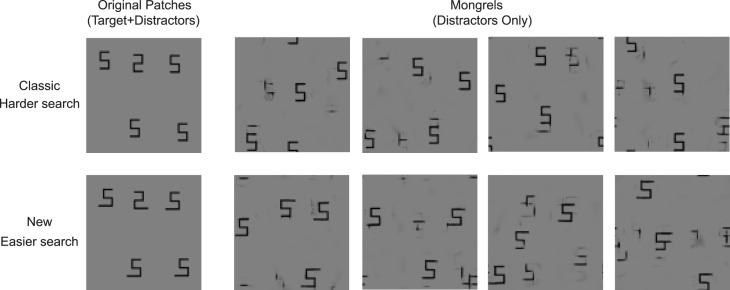
The bottom bar of a 5 has much in common with the top bar, such as similar local orientations and contrast. As a result, the top of one 5 can tile with the bottom of another to make a short chain of “5-stuff.” We frequently see such chains in our mongrels (Figure 2B). Perfectly good 2s appear in the middle of such chains, and in fact, as a result, sometimes appear in the mongrels on their own. This ambiguity about whether target-absent patches contain a target means that tileability explains the difficulty of this classic search condition (20–30 ms/item for target-present trials; Wang, Cavanagh, & Green, 1994; Wolfe, 2007).

Not every lining up of similar things like bars leads to likely tiling. Two 5s do not so easily tile side-by-side, for instance, with the bottom vertical of one lining up with the top vertical of the other. To do so would disagree too much with the image statistics of the original patch; a side-by-side tile of this sort contains significant orientations, coarse-scale spatial frequencies, and pair-wise correlations between orientations (proto-junctions) not present in the original patch. In line with these intuitions, we do not tend to see such side-by-side tiling of 5s in our mongrels.

What if we subtly lengthen the bottom bar of both the 2 and 5 (Figure 5)? The 5s may still tile, but the resulting chain of 5 “stuff” would not contain anything that looks quite like the new target 2 (Figures 3B and 5). Tileability predicts that this subtle modification will make the search task easier. FIT-based search models should predict no difference. Lengthening the bottom bars actually reduces the difference between coarse-scale orientation of the 2 and the 5, so we have actually reduced a potentially informative orientation cue. The new 2 and 5 can still only be differentiated by their spatial configuration.

Figure 5.

Mongrels for 2 among 5 search, old and new conditions. Note the presence of chains with 2-like regions in several of the mongrels for the classic condition (e.g., bottom center of the second mongrel), and the absence of such illusory 2s in the new condition mongrels, as predicted by tileability.

Q among Os

Search for a Q among Os is fairly efficient, whereas search for an O among Qs is inefficient. Classic explanations suggest that it is easier to find the presence of a vertical bar than its absence (Treisman & Souther, 1985).

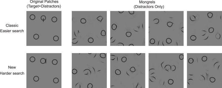
According to tileability, the Q among O search is easy because Os can't easily tile to form a Q. But Os do tile to form a structure that looks like an α (Figures 2C and 6), which is much like the original target Q, but with the bar moved to the side of the O. Tileability predicts that search for an α among Os (Figure 3C) will be more difficult. (For historical reasons, we call these Q among Os tasks, though neither target looks like a Q.)

Figure 6.

Mongrels for Q among O search. Note that, unlike the other conditions, all mongrels shown here come from the same class of original image (i.e., all Os). None of the mongrels (top or bottom) contain strong evidence of a classic Q target, but several contain items that look like alpha or infinity symbols (containing an alpha).

The modified target still contains a unique basic feature, the vertical bar, implying that the stimulus change should have minimal effect, according to classic explanations. The vertical bar remains quite distinct. However, a more detailed account of Q among O search has hypothesized at least four candidate basic features which are unique to the Q: orientation, size/length, intersection, and line termination (Wolfe & Horowitz, 2004). Our modified search task removes an X-junction, adds some other kind of junction, and reduces the size difference between target and distractors. Depending upon one's favorite feature that drives easy Q among O search, classic models may or may not predict more difficult search in the modified condition. Nonetheless we can use this condition to further test the predictive ability of the tileability rule of thumb.

O among Qs

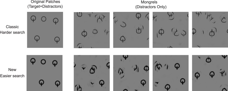
According to tileability, search for an O among Qs may be difficult because the distractors fail to cohere, dispersing into pieces that look like a target O. Perhaps if we render the Os and Qs with thicker lines, we can increase the grouping between the vertical bar and the O. Essentially more scales will signal that the bar co-occurs with the O. Stronger Q coherence should make it easier to disambiguate whether a peripheral patch contains an O, making search easier (Figures 3D and 7). It is difficult to see how making the strokes modestly thicker would change the prediction of classic search models.

Figure 7.

Mongrels for O among Q search, old and new conditions. Note the appearance of several O-like structures in the mongrels for the classic condition (top), but not in the new condition (bottom).

Conjunction search

What about conjunction search? At first it seems nonobvious how one can tile light-vertical and dark-horizontal bars to make a dark-vertical bar. Conjunction search reveals an important aspect of tileability. Tileability derives from the texture tiling model, which computes image statistics on the responses of a multiscale steerable pyramid (Portilla & Simoncelli, 2000; Balas et al., 2009; Rosenholtz et al., 2012a; Rosenholtz et al., 2012b). As a result, one should think of tiling in multiscale subbands, i.e., as acting on the outputs of bandpass filters rather than on the pixels.

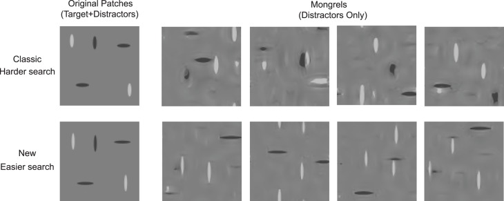
Figure 8 gives intuitions in the 1-D case. It shows two bars, the left one with a positive sign of contrast, and the right with a negative sign of contrast. Below that, we show the results of filtering each bar with a bandpass filter, which computes essentially a blurred second derivative. In a fine-scale subband (left)—where the filter is narrower than the bars—the responses to light bars can tile to make the response to a target dark bar. At scales finer than the bars, we expect illusory conjunctions. In a coarse-scale subband (right)—where the center lobe of the filter is at least as wide as the bar—the responses to light vertical bars cannot easily tile to form the response to a dark vertical target. Scales of processing that are coarse relative to the width of the bars can tell dark bars from light, but finer scales cannot. We are left with a surprising prediction: assuming a limited number of scales of processing, the width of the bars should matter. With fatter bars, more processing scales will be fine relative to the bar, leading to more illusory conjunctions; with thinner bars, more scales will be coarse relative to the bar, leading to fewer illusory conjunctions. Whereas for O among Qs we predict that making the bars thicker makes search easier, here we predict that making the bars thinner makes search easier. The mongrels for these conditions do in fact seem to bear out this intuition (Figure 9).

Figure 9.

Mongrels for conjunction search, old and new conditions. Target is a black vertical. Note the illusory black verticals in the classic search mongrels, which are absent from the mongrels for the new modified condition.

This analysis might at first glance seem to make the absurd prediction that peripheral vision cannot tell a patch with all light bars from one also containing a dark bar, making search for dark among light difficult. However, again, tileability is simply a rule of thumb to give intuitions about the TTM model. The underlying model only confuses patches with similar image statistics. A patch of only light bars cannot be confused with a patch with a dark bar, because the two would have different image statistics, such as the mean luminance. We expect no illusory black bars in a peripheral patch of all light bars. Tiling must preserve the local image statistics measured by the model.

Given that both the classic and modified conjunction tasks (Figure 3E) contain strongly oriented stimuli—the observer should have no difficulty distinguishing horizontal from vertical—it is difficult to see how this subtle manipulation could affect the classic search explanation.

Summary

Through discussion of each of these search conditions, we hope to have given the reader intuitions about the tileability rule of thumb. Two image regions can join or tile if they have contain similar local orientations, so long as their joining does not change the summary contents of the patch as a whole (T among Ls, 2 among 5s, Q among Os). Image regions with (for lack of a better term) weak grouping cues can disperse, particularly if the locations where the parts join in the original contain features similar to those at other locations in the patch. For example, the Qs in the original O among Qs condition contain horizontal + vertical orientation, but so do Os themselves. Although in many cases we can get intuitions by thinking about tiling as occurring on the pixels of the image, more correctly it occurs within multiscale subbands (conjunction search).

We carried out five classic search tasks and their corresponding modified versions using two experimental paradigms. First, we measured the time (RT) to correctly indicate the presence or absence of a target, as a function of the number of items in the display. In addition, we gave a second set of observers a two-interval forced-choice (2IFC) task requiring them to indicate which of two briefly-presented displays contained the target, and measured their performance. We used both paradigms because the RT paradigm represents the standard for the visual search field, but is potentially subject to speed-accuracy tradeoffs.

Search difficulty for new and classic tasks

Methods

Subjects

Six adults participated in each condition after giving written informed consent. One set of six did the O among Q, Q among O, and conjunction search tasks, while another set of six did the other four tasks. In both cases, subjects were aged 18–40 years, half of them male. All subjects reported normal or corrected-to-normal vision and received monetary compensation for their participation. All subjects were naïve as to the purpose of the experiment and were paid for their participation.

Stimuli

In both experiments, the targets and distractors were the same, with one exception: conjunction search with black and white search items (gray values of 0 and 255, respectively) led to performance at ceiling in the 2IFC task. Conjunction search is typically only modestly more difficult than feature search, and less difficult than configuration search. Since we want to test whether making the bars thinner makes search easier, we need to get performance on the classic task off of ceiling. Rather than reducing the display time for these conditions, we instead make the tasks more difficult by reducing the contrast of the display items, setting their gray values to 64 and 192, respectively, instead of to 0 and 255. Stimuli were presented on a 26.8 × 21.1 cm monitor, with subjects seated 75 cm away in a dark room. The search displays consisted of a number of items, either all distractors (target-absent display) or one target and the rest distractors (target-present display). Stimuli were randomly placed on four concentric circles, with added positional jitter (up to 1/8 degree), to minimize accidental alignment of the items. The radii of the circles were 4°, 5.5°, 7°, and 8.5° of visual angle. Each target or distractor subtended approximately 1°. Sample target-present stimuli for two of the conditions, O among Qs and T among Ls, are shown in Figure 10, for set size = 18.

Figure 10.

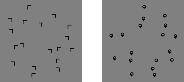
Example layout of search displays. Shown for set size = 18, target-present. Left, search for an upright T among Ls of two possible orientations (our nominal classic search condition). Right, new O among Q search.

Reaction time task

Subjects indicated with a key press whether or not the stimulus contained a target, and were given auditory feedback. The search display appeared on the computer screen until participants responded. Target-present and target-absent displays occurred with equal probability.

Trials were blocked by condition. At the start of each block, participants performed 18 test trials to familiarize them with the target, distractor, and experimental procedure. Each participant completed 216 trials for each task for each condition (108 target-present and 108 target-absent), evenly distributed across three set sizes (6, 12, and 18). The order of testing for classic versus modified conditions was counterbalanced across participants, with half of participants seeing classic conditions first, and half seeing modified conditions first.

2IFC task

On each trial, the participant viewed the first search display for 100 ms, followed by a blank display with a central fixation disk for 500 ms, and then the second search display, also for 100 ms, followed by another blank display (Figure 11). Set size was always 18. One of the two displays was always target-present, and the other was target-absent. Target-present displays appeared first or second with equal probability. Participants gave a nonspeeded response, indicating with a key press whether the first or second display contained the target. They received auditory feedback as to the correctness of their answer.

Figure 11.

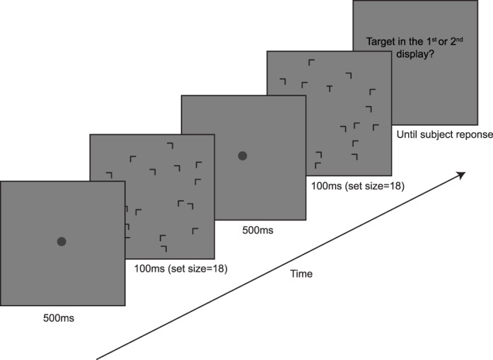
A 2IFC trial. Target-present in the second display. All 2IFC trials had set size = 18.

Each participant performed 72 trials in each of the 10 experimental conditions. The order in which subjects saw classic versus modified conditions was counterbalanced across subjects. Before each task, subjects had 12 practice trials to become familiar with the target, distractor, and the procedure.

Results

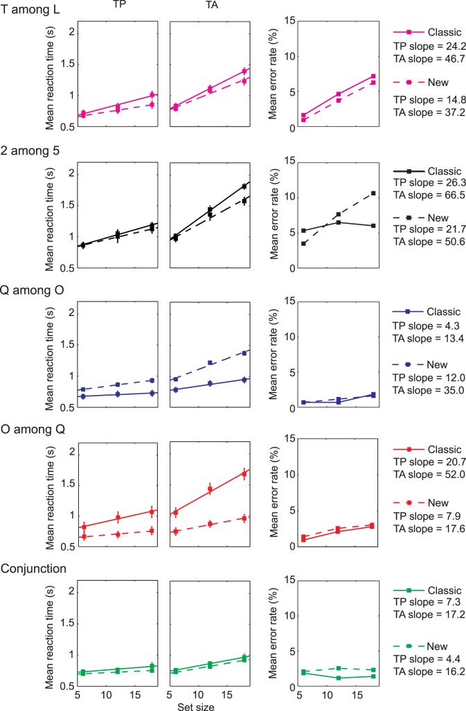
Figure 12 plots mean reaction time versus set size for correct target-present and target-absent trials, from the RT tasks. Mean RTs were estimated using log-transformed data, as in Zhou and Gao (1997). As is standard in the search literature, we quantify search difficulty as the slope of the best-fit line (also shown). The legend for each search task gives the target-present and target-absent slopes. Figure 12 also shows average error rates for each combination of set size and search condition. Experimental results for the classic search conditions were consistent with previously reported studies.

Figure 12.

Results from the reaction time task. Reaction times versus set size for correct target-present (TP) and target-absent (TA) trials, along with error rates, averaged across subjects. Error bars show standard errors. Solid lines represent linear fits for classic search experiments. Dashed lines are fits to data for the new modified tasks. Slopes are given in the legend.

In the rest of the analysis and discussion of the RT tasks we focus on correct target-present slopes. Many models of search, including TTM, predict a similar relationship between target-present and target-absent slopes. Typical target-absent trials are inherently slower due to a need to make decisions about all noisy items in the display, as opposed to needing to make decisions about only half of the items, on average, in a target-present display. This holds true not only for serial models like FIT, but also for parallel models (e.g., Chen, Navalpakkam, & Perona, 2011), as well as models that employ a combination of serial and parallel processing. In fact, one can see little of interest in the target-absent data, with the slopes generally about twice that of target present trials. Furthermore, target-absent trials can be governed by criterion setting issues, often orthogonal to the question at hand.

The rightmost column of Figure 13 summarizes the experimental results from both the RT tasks and the 2IFC tasks. For each condition, the direction of the arrow indicates whether tileability predicts that the modified search task will be easier or harder than the classic task. Search difficulties for the 2IFC test are characterized by error rate. For all five pairs of conditions and both experimental paradigms, search performance changed by a significant amount in the direction predicted by tileability.

Figure 13.

Predictions of tileability versus experimental results. Left column shows targets and distractors for each condition. Middle column summarizes the tileability explanation for new and classic conditions. Right column shows experimental results. Arrows indicate the direction of the predicted change in performance for new versus classic tasks. The two bars on the left indicate RT versus set size slopes for correct target-present trials. A higher slope indicates a harder task. The right two bars give mean error rates in the 2IFC experiment. A higher error rate means a harder search task. In each case, for both the RT and 2IFC experiments, search performance changed significantly in the direction predicted by tileability. Error bars show standard error.

In particular, tileability correctly predicts that looking for an upright T (0°) among distractors (L₀, L₉₀) is easier than looking for the upright T among distractors (L₉₀, L₁₈₀). As predicted, the slope of the modified task is significantly shallower than that of the classic: slope difference = −9.4 msec/item; one-tailed paired t test, t(5) = −3.69, p = 0.007. These results were consistent with the 2IFC tasks: difference in error rate = −11.8%; one-tailed paired t test, t(5) = −4.09, p = 0.005.

We predicted that a modest lengthening of one of the bars on both the 2 and 5 would make that search easier. In fact, search was significantly more efficient in the modified condition: slope difference = −4.7 msec/item; one-tailed paired t test, t(5) = −2.17, p = 0.041. Error rates on the 2IFC task for the modified condition were also significantly lower: difference = −5.5%; one-tailed paired t test, t(5) = −2.11, p = 0.004.

For Q among O search, tileability predicted that simply moving the position of the vertical line in the Q would make this easy task more difficult. The experimental results of both RT and 2IFC tests confirmed this prediction. The modified search task is significantly less efficient: slope difference = 7.7 msec/item; one-tailed paired t test, t(5) = 2.50, p = 0.027, and led to significantly poorer performance on the 2IFC task: difference in error rate = 12.5%; one-tailed paired t test, t(5) = 2.96, p = 0.016.

We predicted that search for an O among Qs becomes easier when one makes the lines thicker. Search was significantly more efficient in the modified condition: mean difference in slope = −12.8 msec/item; one-tailed paired t test, t(5) = −6.36, p = 0.001. The results of the 2IFC experiment further validate this conclusion, as participants made significantly fewer errors in the modified O among Qs search task: mean difference in error rate = −7.6%; one-tailed paired t test, t(5) = −3.91, p = 0.006.

Finally, tileability predicted that we could reduce the number of illusory conjunctions, and thus make conjunction search easier, by making the bars thinner. The experimental results echoed our predictions, with shallower search slope: slope difference = −2.9 msec/item; one-tailed paired t test, t(5) = −2.31, p = 0.034 in the reaction time paradigm, and lower error rates: difference = −6.7%; one-tailed paired t test, t(5) = −2.51, p = 0.027 in the 2IFC paradigm.

It is difficult to see how such modest, image-based changes, such as moving basic features, or making bars thicker, thinner, or longer, would lead to changes in performance, if the presence or absence of a basic feature was the principle underlying search difficulty.

Discussion

Traditional models of visual search have suggested that a key factor determining task difficulty consists of whether or not the search target contains a basic feature not found in the distractors. Recently we extended our texture tiling model of peripheral encoding to search. This model puts the blame for many difficult search tasks not on the limits of preattentive vision, but rather on the limits of peripheral vision. If peripheral vision loses too much information, it will be difficult to tell apart a target-present patch from a target-absent patch; search will be difficult. Both the traditional FIT and TTM can explain a number of classic search results. Here we attempt to directly discriminate between the two models. Our results were better predicted by TTM than by FIT.

It is worth noting that TTM itself has limits. For instance, it almost certainly cannot predict the asymmetry in which search for a tilted line among vertical is easier than vice versa. However, others have predicted this asymmetry essentially by adding a component to the model (Heinke & Backhaus, 2011; Vincent, 2011; see also discussion in Rosenholtz et al., 2012a), and this seems also a plausible solution for TTM. A later version of TTM might also include additional image statistics; it currently has no explicit end-stopping, which might be required for adequate performance on a C among Os task, and it also currently lacks correlations across space between different orientations, perhaps necessary for good continuation. Furthermore, future work is required to incorporate TTM into a more complete model of search, including predicting reaction times, choosing stopping criteria, and utilizing priors about target location.

FIT has long benefited (and arguably also suffered) from having an intuitive word model. Researchers may find such models lead to easier intuitions, enabling design of novel experiments to test the theory. Similarly, Duncan and Humphreys (1989) related increased search efficiency to both increasing target-distractor similarity and decreasing distractor-distractor similarity. Though they only fairly vaguely defined “similarity” and the template-matching and grouping processes presumed to underlie the observed effects, this work has been highly cited and inspired much research, particularly on heterogeneity effects. Quite possibly the peripheral crowding mechanisms modeled by TTM underlie the similarity effects described by Duncan and Humphreys (1989). For instance, their suggestion that similarity might have to do with the amount of shared contour might sound related to aspects of tileability. Furthermore, strength of crowding is known to depend both upon target-flanker grouping (Andriessen & Bouma, 1976; Kooi, Toet, Tripathy, & Levi, 1994; Saarela, Sayim, Westheimer, & Herzog, 2009) and flanker-flanker grouping (Livne & Sagi, 2007; Sayim, Westheimer, & Herzog, 2010; Manassi, Sayim, & Herzog, 2012).

To gain easier intuitions about TTM, we developed a rule of thumb for that model, which we call tileability. Crowding in peripheral vision leads to ambiguities between an original patch and jumbled versions of that patch. If in that jumbling, distractors can easily tile produce a target, search is hard. Similarly, if in that jumbling the distractors disperse and form the target, search is hard. We hope that tileability provides researchers with an intuitive shortcut to predictions of TTM. Of course, tileability can provide only qualitative predictions (one condition is easier than another) rather than more quantitative predictions (how much easier).

Ultimately, however, TTM is the true model. TTM computes image statistics on the responses of a multiscale steerable pyramid. TTM only confuses patches with similar image statistics. This means that while we can gain a certain amount of leverage by imagining tiling in the image domain, ultimately tiling “occurs” in subbands, operating on the outputs of bandpass filters, not on pixels, nor on presegmented entities like bars. Tiling does not produce a random pileup of distractors; only local regions with similar responses to oriented filters are likely to tile together to form new structures. The jumbled patch as a whole must preserve the image statistics of the original patch. If there is any question as to the predictions of TTM, one can use our standard methodology of generating mongrels from target-present and target-absent patches, and measuring discriminability of those mongrels (Rosenholtz et al., 2012b; Zhang et al., 2015). Unlike FIT or similarity theory, our word model has a clearly defined computational model to back it up.

In this paper, we compared FIT and TTM by testing performance on new search tasks. Five classic search tasks—explained by both TTM and the traditional FIT model—form the basis for these new search experiments.

Based on tileability, we modified each of these search tasks in a way that should make minimal difference to FIT, but matter to TTM. In each case, tileability made predictions in advance about whether the modifications would make search easier or harder. We then ran both standard RT search tasks and a 2IFC version, and looked at which theory does better. Experimental results from both RT tasks and 2IFC tasks show that fairly subtle changes in these search tasks lead to significant changes in performance, in a direction predicted by tileability. Classic search models do not obviously predict these results. At the very least, the effects of subtle stimulus changes point to the need for models that operate on images, rather than on presegmented “things,” like bars. Furthermore, the success of tileability provides definitive evidence in favor of the texture tiling model explanation of search as opposed to FIT.

References

- Alexander R. G,, Schmidt J,, Zelinsky G. J. (2014). Are summary statistics enough? Evidence for the importance of shape in guiding visual search. Vision Cognition, 22 (3–4), 595–609. doi:10.1080/13506285.2014.890989. [DOI] [PMC free article] [PubMed] [Google Scholar]
- Andriessen J. J,, Bouma H. (1976). Eccentric vision: Adverse interactions between line segments. Vision Research, 16, 71–78. [DOI] [PubMed] [Google Scholar]
- Balas B. J,, Nakano L,, Rosenholtz R. (2009). A summary statistic representation in peripheral vision explains visual crowding. Journal of Vision, 9 (12): 13 1–18. doi:10.1167/9.12.13 [PubMed] [Article] [DOI] [PMC free article] [PubMed] [Google Scholar]
- Bergen J. R,, Julesz B. (1983). Rapid discrimination of visual patterns. IEEE Transactions on Systems, Man, and Cybernetics, SMC-13, 857–863.
- Bouma H. (1970). Interaction effects in parafoveal letter recognition. Nature, 226, 177–178. [DOI] [PubMed] [Google Scholar]
- Carrasco M,, Evert D. L,, Chang I,, Katz S. M. (1995). The eccentricity effect: Target eccentricity affects performance on conjunction searches. Perception & Psychophysics, 57, 1241–1261. [DOI] [PubMed] [Google Scholar]
- Carrasco M,, McLean T. L,, Katz S. M,, Frieder K. S. (1998). Feature asymmetries in visual search: Effects of display duration, target eccentricity, orientation and spatial frequency. Vision Research, 38, 347–374. [DOI] [PubMed] [Google Scholar]
- Carrasco M,, Yeshurun Y. (1998). The contribution of covert attention to the set-size and eccentricity effects in visual search. Journal of Experimental Psychology: Human Perception and Performance, 24, 673–692. [DOI] [PubMed] [Google Scholar]
- Chen B,, Navalpakkam V,, Perona P. (2011). Predicting response time and error rate in visual search. Shawe-Taylor J,, Zemel R. S,, Bartlett P. L,, Pereira F,, Weinberger K. Q. (Eds.), Advances in neural information processing systems (pp 2699–2707). Granada, Spain: NIPS Foundation. [Google Scholar]
- Duncan J,, Humphreys G. W. (1989). Visual search and stimulus similarity. Psychological Review, 96, 433–458. [DOI] [PubMed] [Google Scholar]
- Ehinger K. A,, Rosenholtz R. (2016). Peripheral information loss predicts human performance on a range of scene-perception tasks relevant for navigation. Manuscript submitted for publication.
- Freeman J,, Simoncelli E. P. (2011). Metamers of the ventral stream. Nature Neuroscience, 14 (9), 1195–1201. [DOI] [PMC free article] [PubMed] [Google Scholar]
- Heinke D,, Backhaus A. (2011). Modeling visual search with the selective attention for identification model (VS-SAIM): A novel explanation for visual search asymmetries. Cognitive Computation, 3, 185–205. [DOI] [PMC free article] [PubMed] [Google Scholar]
- Hulleman J,, Olivers C. N. L. (2015). The impending demise of the item in visual search. Behavioral and Brain Sciences, 1, 1–76. doi:10.1017/S0140525X15002794. [DOI] [PubMed] [Google Scholar]
- Keshvari S,, Rosenholtz R. (2016). Pooling of continuous features provides a unifying account of crowding. Journal of Vision, 16 (3): 13 1–15. doi:10.1167/16.3.39 [PubMed] [Article] [DOI] [PMC free article] [PubMed] [Google Scholar]
- Kooi F. L,, Toet A,, Tripathy S. P,, Levi D. M. (1994). The effect of similarity and duration on spatial interaction in peripheral vision. Spatial Vision, 8, 255–279. [DOI] [PubMed] [Google Scholar]
- Korte W. (1923). Über die Gestaltauffassung im indirekten Sehen [Translation: On the apprehension of Gestalt in indirect vision]. Zeitschrift für Psychologie, 93, 17–82. [Google Scholar]
- Lettvin J. Y. (1976). On seeing sidelong. The Sciences, 16 (4), 10–20. [Google Scholar]
- Livne T,, Sagi D. (2007). Configuration influence on crowding. Journal of Vision, 7 (2): 13 1–12. doi:10.1167/7.2.4 [PubMed] [Article] [DOI] [PubMed] [Google Scholar]
- Manassi M,, Sayim B,, Herzog M. (2012). Grouping, pooling, and when bigger is better in visual crowding. Journal of Vision, 12 (10): 13 1–14. doi:10.1167/12.10.13 [PubMed] [Article] [DOI] [PubMed] [Google Scholar]
- Oliva A,, Torralba A,, Castelhano M. S,, Henderson J.M. (2003). Top-down control of visual attention in object detection. Proceedings of the IEEE International Conference on Image Processing, 1, 253–256. [Google Scholar]
- Oliva A,, Wolfe J. M,, Arsenio H. (2004). Panoramic search: The interaction of memory and vision in search through a familiar scene. Journal of Experimental Psychology: Human Perception and Performance, 30, 1132–1146. [DOI] [PubMed] [Google Scholar]
- Pelli D. G,, Palomares M,, Majaj N. (2004). Crowding is unlike ordinary masking: Distinguishing feature integration from detection. ournal of Vision, 4 (12): 13, 1136–1169. doi:10.1167/4.12.12 [PubMed] [Article] [DOI] [PubMed] [Google Scholar]
- Portilla J,, Simoncelli E. (2000). A parametric texture model based on joint statistics of complex wavelet coefficients. International Journal of Computer Vision, 40, 49–71. [Google Scholar]
- Reddy L,, VanRullen R. (2007). Spacing affects some but not all visual searches: Implications for theories of attention and crowding. Journal of Vision, 7 (2): 13 1–17. doi:10.1167/7.2.3 [PubMed] [Article] [DOI] [PubMed] [Google Scholar]
- Rosenholtz R,, Huang J,, Ehinger K. A. (2012a). Rethinking the role of top-down attention in vision: Effects attributable to a lossy representation in peripheral vision. Frontiers in Psychology, 3, 1–15. [DOI] [PMC free article] [PubMed] [Google Scholar]
- Rosenholtz R,, Huang J,, Raj A,, Balas B. J,, Ilie L. (2012b). A summary statistic representation in peripheral vision explains visual search. Journal of Vision, 12 (4): 13 1–17. doi:10.1167/12.4.14 [PubMed] [Article] [DOI] [PMC free article] [PubMed] [Google Scholar]
- Saarela T. P,, Sayim B,, Westheimer G,, Herzog M. H. (2009). Global stimulus configuration modulates crowding. Journal of Vision, 9 (2): 13 1–11. doi:10.1167/9.2.5 [PubMed] [Article] [DOI] [PubMed] [Google Scholar]
- Sayim B,, Westheimer G,, Herzog M. H. (2010). Gestalt factors modulate basic spatial vision. Psychological Science, 21, 641–644. [DOI] [PubMed] [Google Scholar]
- Treisman A,, Gelade G. (1980). A feature-integration theory of attention. Cognitive Psychology, 12, 97–136. [DOI] [PubMed] [Google Scholar]
- Treisman A,, Souther J. (1985). Search asymmetry: A diagnostic for preattentive processing of separable features. Journal of Experimental Psychology: General, 114, 285–310. [DOI] [PubMed] [Google Scholar]
- Vincent B. (2011). Search asymmetries: Parallel processing of uncertain sensory information. Vision Research, 51, 1741–1750. [DOI] [PubMed] [Google Scholar]
- Vlaskamp B. N. S,, Over E. A. C,, Hooge I. T. C. (2005). Saccadic search performance: The effect of element spacing. Experimental Brain Research, 167, 246–259. [DOI] [PubMed] [Google Scholar]
- Wang Q,, Cavanagh P,, Green M. (1994). Familiarity and pop-out in visual search. Perception & Psychophysics, 56, 495–500. [DOI] [PubMed] [Google Scholar]
- Wertheim A. H,, Hooge I. T. C,, Krikke K,, Johnson A. (2006). How important is lateral masking in visual search? Experimental Brain Research, 170, 387–401. [DOI] [PubMed] [Google Scholar]
- Wolfe J. M. (1994). Guided Search 2.0: A revised model of visual search. Psychonomic Bulletin & Review, 1, 202–238. [DOI] [PubMed] [Google Scholar]
- Wolfe J. M. (2001). Asymmetries in visual search: An introduction. Perception & Psychophysics, 63, 381–389. [DOI] [PubMed] [Google Scholar]
- Wolfe J. M. (2007). Guided Search 4.0: Current progress with a model of visual search. Gray W. (Ed.) Integrated models of cognitive systems (pp 99–119). New York, NY: Oxford. [Google Scholar]
- Wolfe, J. M,, Butcher S. J,, Lee C,, Hyle M. (2003). Changing your mind: On the contributions of top-down and bottom-up guidance in visual search for feature singletons. Journal of Experimental Psychology: Human Perception and Performance, 29 (2), 483–503. [DOI] [PubMed] [Google Scholar]
- Wolfe J. M,, Horowitz T. S. (2004). What attributes guide the deployment of visual attention and how do they do it? Nature Reviews Neuroscience, 5, 495–501. [DOI] [PubMed] [Google Scholar]
- Wolfe J. M,, Horowitz T. S,, Kenner M. (2005). Rare items are often missed in visual searches Nature, 435, 439–440. [DOI] [PMC free article] [PubMed] [Google Scholar]
- Zhang X,, Huang J,, Yigit-Elliott S,, Rosenholtz R. (2015). Cube search, revisited. Journal of Vision, 15 (3): 13 1–18. doi:10.1167/15.3.9 [PubMed] [Article] [DOI] [PMC free article] [PubMed] [Google Scholar]
- Zhou X.-H,, Gao S. (1997). Confidence intervals for the log-normal mean. Statistics in Medicine, 16, 783–790. [DOI] [PubMed] [Google Scholar]
Associated Data
This section collects any data citations, data availability statements, or supplementary materials included in this article.