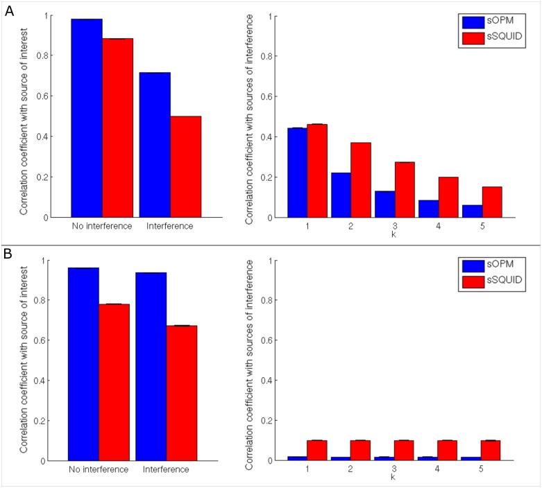
Fig 5. Reconstruction accuracy with “brain noise”.
(A) Case 1 (interference in close proximity): left hand panel shows average of correlation coefficients between simulated and reconstructed dipole time courses, r(qj,q̂j), with and without interference. Right hand panel shows average of correlation coefficients between each of the interference sources and the reconstructed main dipole time course, i.e. rInt(qInt,k,q̂j). (B) Case 2 (deep sources): left hand panel represents the average of correlation coefficients between the estimated and the simulated dipole time course, with and without interference sources. Right hand panel shows again average of correlation coefficients with sources of interference.

