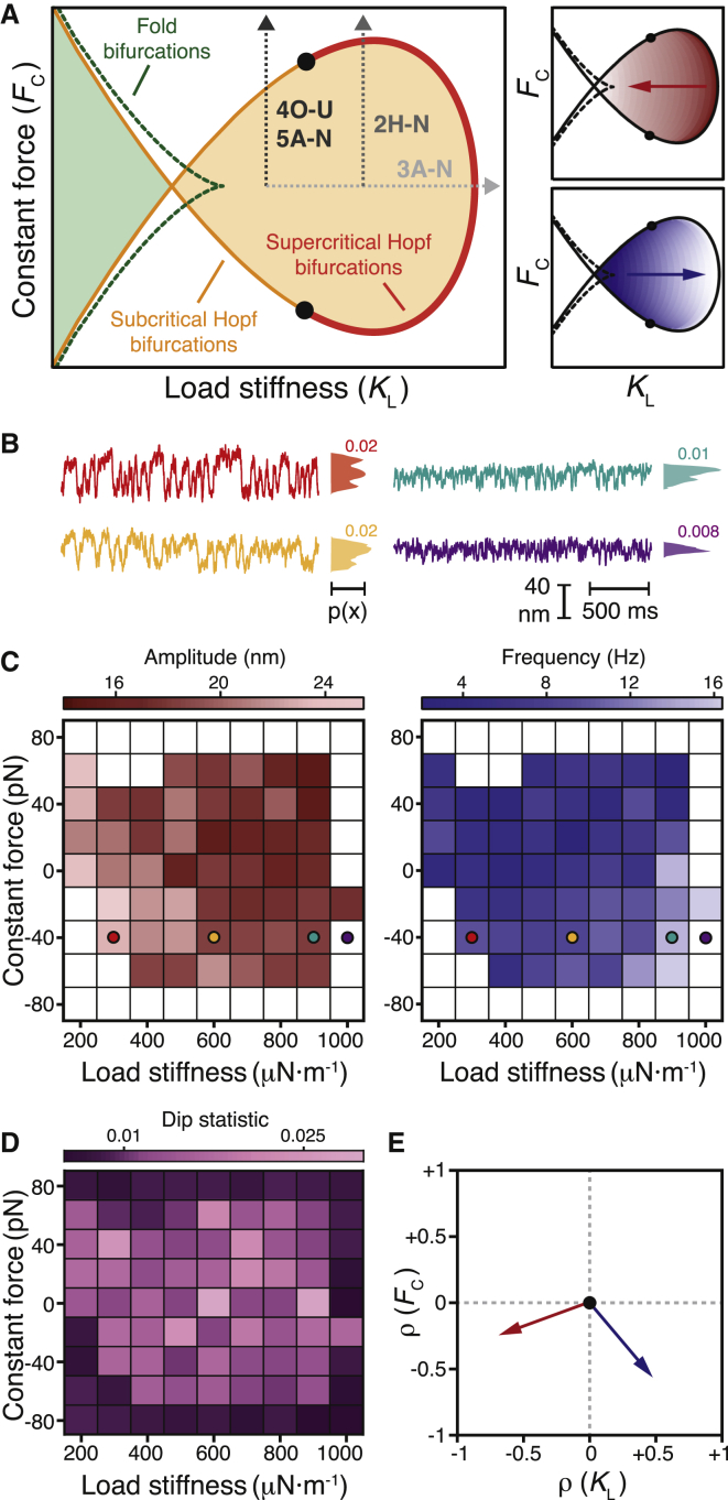
Figure 1.

Hair-bundle state diagram. (A) A theoretical state diagram specifies the behaviors of a hair bundle for various combinations of constant force (F_C) and load stiffness (K_L). A line of Hopf bifurcations (red) separates a region within which a hair bundle oscillates spontaneously (orange) from one in which the bundle remains quiescent (white). Bautin points (black) lie at the border between the supercritical and subcritical segments of this line. Within the spontaneously oscillatory region, a bundle’s oscillations fall in amplitude and rise in frequency with an increase in load stiffness (red and blue arrows, right panels). A line of fold bifurcations (green, dashed) confines a region within which a bundle exhibits bistability (light green). The gray arrows correspond to the regions of the bundle’s state diagram explored in Figs. 2, 3, 4, and 5. (B) Oscillations of an experimentally observed hair bundle changed in appearance as the load stiffness increased from 300 μN⋅m⁻¹ to 1000 μN⋅m⁻¹ (red to purple). The position histograms and associated dip statistics shown to the right of each trace signal the presence or absence of spontaneous oscillations. The dip statistic quantifies the modality of the system’s position histogram; a dip statistic of at least 0.01 with p < 10⁻³ implies spontaneous oscillation. (C) An experimental state diagram depicts the behavior of a hair bundle for different values of the load stiffness and constant force. White boxes correspond to operating points at which the bundle’s position histogram possessed a dip statistic of <0.01, indicating quiescent behavior. Within the territory of spontaneous oscillation, the intensities of red and blue correspond to the amplitude and frequency, respectively, of the bundle’s oscillations calculated with a peak-detection algorithm with a threshold of 25 nm. Colored circles correspond to the traces in (B). (D) The dip-statistic values for the experimental state diagram in (C) are displayed in shades of purple. (E) Spearman’s rank correlation (ρ) quantifies the relationships between amplitude (red arrow) and frequency (blue arrow) with the load stiffness (ρ(K_L)) and constant force (ρ(F_C)) (Table S1). For all experimental data, the stiffness and drag coefficient of the stimulus fiber were k_SF = 109 μN⋅m⁻¹ and ξ_SF = 142 nN⋅s⋅m⁻¹, respectively. The proportional gain of the load clamp was 0.01. For a complete description of the bundle’s experimental state diagram, see Supporting Material Section B.