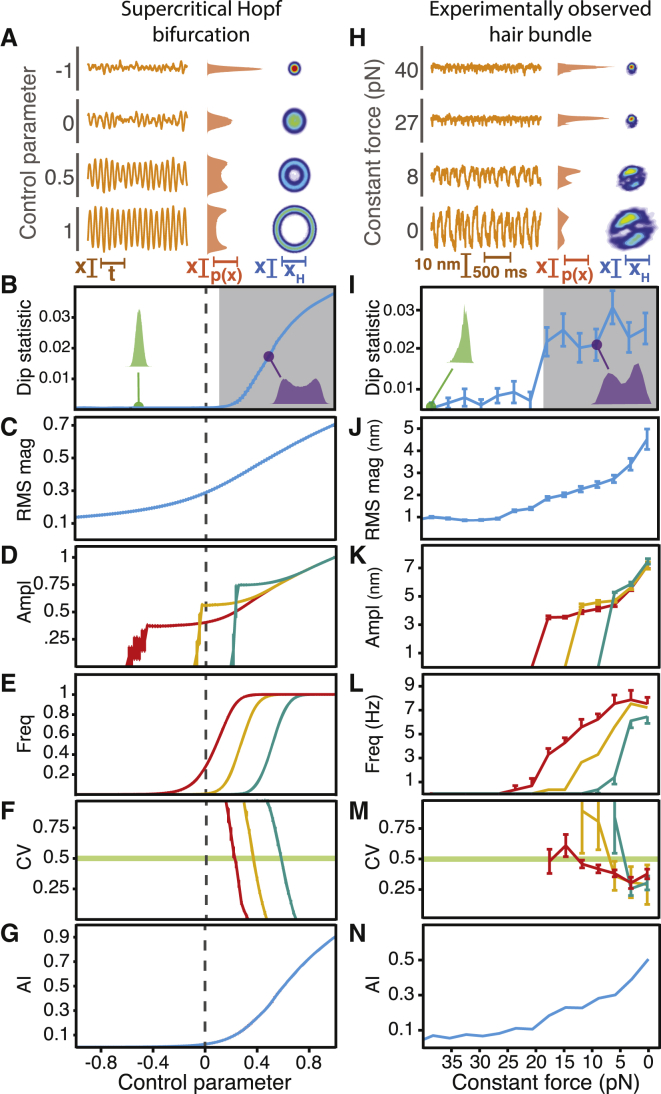
Figure 2.
Crossing a supercritical Hopf bifurcation by adjusting the constant force. (A–N) Over a range of parameter values, we compared the behavior near a supercritical Hopf bifurcation with additive noise (A–G) with that of an experimentally observed hair bundle (H–N). (A) A noisy system operating near a supercritical Hopf bifurcation displayed noise-induced ringing when the control parameter was negative, but oscillated spontaneously for positive values (left). When the amplitude of spontaneous oscillation surpassed that of the noise, the position histogram (middle) disclosed two peaks. When the control parameter exceeded zero, the joint probability distribution (right) for each real-valued position (X) and its Hilbert transform (XH)—the analytic distribution—was circular, with a diameter that grew with the control parameter. In all of the analytic distributions, red and blue correspond to high and low probability values, respectively. Probabilities of or near zero are displayed in white. (B) The dip statistic for the position distribution is shown as a function of the control parameter. A low value for the dip statistic corresponded to a unimodal distribution (green). When the control parameter exceeded zero and the amplitude of oscillation exceeded the level of the noise, the position histogram displayed two peaks (purple) corresponding to a large value of the dip statistic. The control parameter value at which the dip statistic achieved significance (shaded; p < 10−3) served as an estimate of the bifurcation’s location (dashed line). (C) The RMS magnitude of the system’s motion rose gradually as the control parameter increased. (D) The amplitude rose with the control parameter for peak-detection thresholds of 0.68 (red), 1.06 (yellow), and 1.45 (cyan). (E) The frequency of oscillation, with the same thresholds as in (D), grew with an increase in the control parameter until it achieved a constant value. The value of the control parameter at which the rise in frequency was steepest increased with the threshold. (F) The coefficient of variation describes the regularity of oscillation, with a high value corresponding to increased variability in the interpeak time interval. The value of the control parameter at which the coefficient of variation crossed 0.5 increased with the peak-detection threshold. (G) The analytic information rose gradually with the control parameter. (H) The behavior of an experimentally observed hair bundle was transformed by changes in the constant force: as the force decreased, the amplitude of spontaneous oscillation rose (left) and the position histogram became bimodal (middle). The analytic distribution formed a loop whose diameter increased with a decrease in the constant force (right). (I) Reflecting a unimodal position histogram, the dip statistic remained small for large values of the constant force (green). When the constant force fell below 20 pN, the position histogram displayed two peaks (purple) and the dip statistic increased, defining the boundary of an oscillatory regime (shaded; p < 10−3). (J) The RMS magnitude of the bundle’s motion rose gradually as the constant force decreased. (K) The amplitude increased as the constant force declined for peak-detection thresholds of 6 nm (red), 8 nm (yellow), and 10 nm (cyan). (L) The frequency of oscillation rose gradually with a decrease in constant force until it achieved a constant value near 5 pN. The force at which this rise in frequency occurred depended on the threshold value. (M) The coefficient of variation exceeded 0.5 at a value of constant force that decreased as the peak-detection threshold increased. (N) The analytic information rose gradually as the constant force fell. For all experimental data, the load stiffness was 400 μN⋅m−1 with a gain of 0.1. The stiffness and drag coefficient of the stimulus fiber were respectively 109 μN⋅m−1 and 142 nN⋅s⋅m−1. All simulations possessed noise with standard deviations of σR = σI = 0.1. The error bars represent the standard errors of the means.

