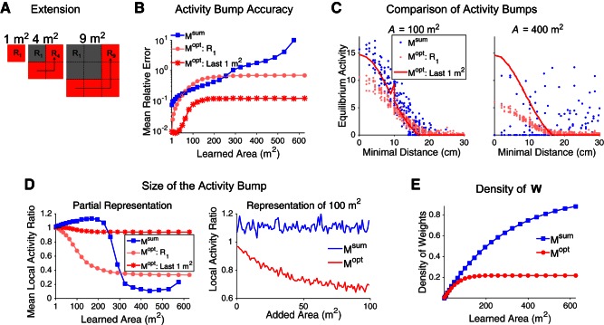
Fig. 9.
Gradual extension of the megamap representing a square environment. A: at each iteration n, the megamap grows from (n − 1)2 m2 to n2 m2 by sequential addition of (2n − 1) subregions of size 1 × 1 m2, from the bottom left to the top right, by Eq. 10 (Mopt) or Eq. 11 (Msum). B: after each iteration n, the equilibrium activity bump is compared with the desired activity (Eq. 9) when the animal is placed at 50 random locations taken throughout the environment for Msum (blue) or within the last subregion learned (Rn2; dark red) or first subregion learned (R1, light red) for Mopt. As the megamap grows, Mopt accurately learns new subregions (dark red) at the cost of previously learned locations (light red). Msum becomes increasingly inaccurate until reaching a breakdown point (∼300 m2) beyond which it can no longer represent any location (blue). C, left: after learning 100 m2, both Msum and Mopt encode any location in the environment through the equilibrium activity bump. Right, after learning 400 m2, Msum no longer has an equilibrium activity bump anywhere in the environment. The amplitude of the equilibrium activity bump of Mopt depends on how recently the location was learned. D: for Mopt, the animal gradually forgets locations previously learned as the megamap grows. Mopt always forms a strong equilibrium activity bump at newly acquired locations (red), but the equilibrium activity bump representing R1 decreases in size as the learned area increases (left; light red). For example, after learning 100 m2, the size of the equilibrium activity bump of Mopt representing any location decreases as a function of the area added to the megamap since learning that location (right). On the other hand, Msum uniformly represents the entire learned region (right; blue). When the learned area becomes sufficiently large, Msum has no equilibrium activity bump, resulting in very little activity near the animal's location (left; blue). The local activity ratio is the ratio of net activity of the equilibrium and desired (Eq. 9) activity bumps, where the activity is summed over all cells with a place field within 10 cm of the animal. E: the density of recurrent connections increases according to Eq. 19 for Msum but approaches 0.25 for Mopt. For all plots, equilibrium activity bumps are computed by setting the input by Eq. 8 with Ipeak = 0.3.

