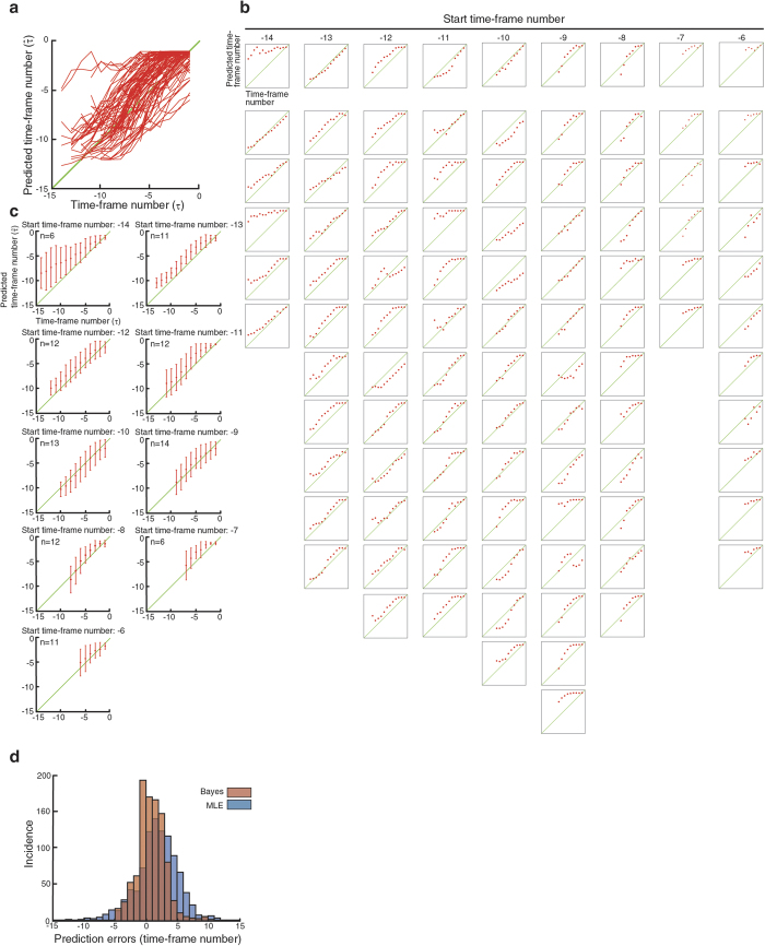
Figure 5. Prediction of the division-timing by sequential Bayesian inference.

(a) Prediction of the division-timing of 97 individual V2 cells. Each line represents the prediction of individual cells. (b) Predictions of each V2 cell are separately shown as dot plot according to their start-point of observations. Each dot in each plot represents the prediction at each time-point. (c) Compilation of the predictions according to their start-point of observations. Average (red dot) and standard deviation (red line) are shown for each time-point. Diagonal line (green) represents the perfect prediction (i.e., the actual division-timing). (d) Comparison of sequential Bayesian inference and MLE methods. Prediction errors for sequential Bayesian inference (red bars) and MLE (blue bars) methods are shown as bar graph. Prediction errors are indicated by the number of time-point deviations from the perfect division-timing prediction (i.e., observed). The superior predictions with sequential Bayes are statistically significant as compared to those with MLE (p = 1.40e⁻²², Mann-Whitney U test).