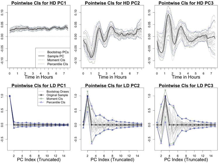
Figure 3.

Bootstrap PC variability - Each column of plots corresponds to a different PC, either the first, second or third. The top row shows the fitted principal components on the original high dimensional space (V_[,k] for k = 1, 2, 3), along with pointwise confidence intervals, and 30 draws from the bootstrap distribution. The bottom row shows the same information, but for the low dimensional representation of the bootstrap PCs ( ${\mathbf{A}}_{[,k]}^b$ for k = 1, 2, 3). In the bottom row, the thick black line corresponds to the case when ${\mathbf{A}}_{[,k]}^b={\mathbf{I}}_{n[,k]}$, where I_n[,k] is the k^th column of the n × n identity matrix, such that ${\mathbf{V}}_{[,k]}^b=\mathbf{V}{\mathbf{A}}_{[,k]}^b={\mathbf{V}}_{[,k]}$.