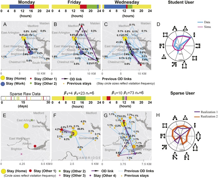
Fig. 4.

Simulation of daily trajectories of one active commuter and one sparse user. (A–C) Simulated trajectories of the student with self-collected cell phone records. Three sample days are shown here. The trips for each sample day are in purple, and the visitation frequency of each location is calculated until the sample day and represented by the circle sizes. (D) Distributions of daily mobility motifs for the active commuter’s data vs. simulation. The model captures well the higher propensity of motifs with node sizes 2 and 3 as well as some other occurrences. (E) A sample sparse user with 10 stays at 4 distinct locations in an observation period of 30 d. (F and G) Two different realizations for simulating the same sparse user with different parameter values. The first realization uses $n_w=6$, ${\beta }_1=4$, ${\beta }_2=23$. The second realization uses $n_w=6$, ${\beta }_1=10$, ${\beta }_2=73$. Larger values of ${\beta }_1$ and ${\beta }_2$ generate more consecutive out-of-home activities and more daily visited locations. (H) Distributions of daily mobility motifs for the two realizations of the same sparse user using different parameter values. With small $n_w$, ${\beta }_1{n}_w$, and ${\beta }_2{n}_w$ values the person is likely to have simple motifs, whereas large parameter values lead to more complex daily activity chains.