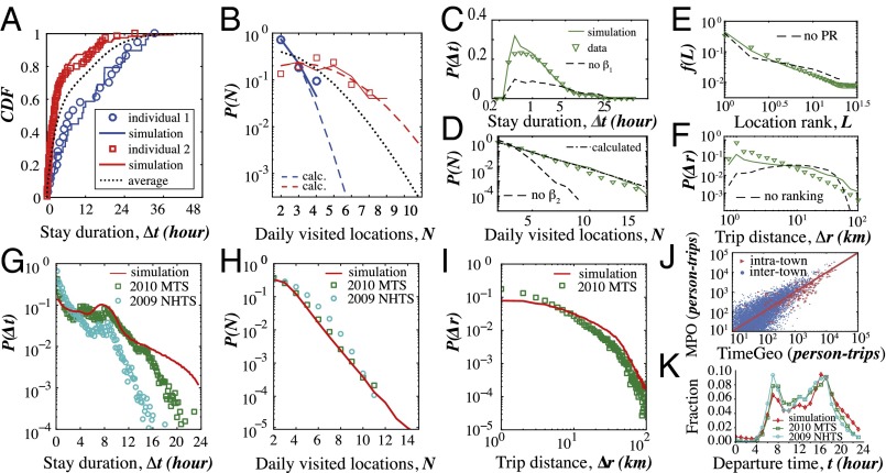
Fig. 5.

Mobility patterns for different individuals and population distributions. The top panels (A–F) show the comparison of the simulation results with the phone data for noncommuters. (A and B) Comparison of mobility patterns for three representative noncommuters. Individuals 1 and 2 represent two extreme cases, one has shorter stays (shown in squares, $n_w=10.86$, ${\beta }_1=6$, ${\beta }_2=41$) and the other travels less frequently (shown in circles, $n_w=5.51$, ${\beta }_1=1$, ${\beta }_2=36$). The third case represents an average noncommuter and is simulated using the median parameter values of $n_w$, ${\beta }_1$, and ${\beta }_2$. (A) Stay duration distribution. (B) Daily visited location distribution. The Markov modeling framework allows the calculations of the number of visited locations per day, as shown in dashed lines, and is discussed in SI Appendix. (C) Activity duration distribution $P\left(\mathrm{\Delta }t\right)$. The model without differentiating home and other states (setting ${\beta }_1=1$) is considered as a benchmark here. In this case, stays with short duration are underestimated. (D) The distribution of the number of daily visited location $P\left(N\right)$. Both the model’s calculation and simulation results are shown. It shows the need for the ${\beta }_2$ parameter in the model. (E) Visitation frequency $f\left(L\right)$ to the Lth most visited location follows the form $f\left(L\right)\sim L^{-1.2\mathrm{\pm }0.1}$. The benchmark shows the result without the preferential return mechanism. (F) Trip distance distribution $P\left(\mathrm{\Delta }r\right)$ extracted from data, and simulation results using an r-EPR mechanism, compared with the random selection of exploration locations (not using the rank-based selection mechanism). The bottom panels (G–K) show the comparison of the simulated daily mobility patterns for the population (aged 16 and over, for both commuters and noncommuters) in Metro Boston (3.54 million individuals) with traditional travel survey data, including the 2009 NHTS, and the 2010–2011 MTS. (G) Stay duration distribution. (H) Daily visited location distribution. (I) Trip distance distribution. (J) Comparison of total commuting trips between and within the 164 cities and towns (i.e., inter- and intratown) estimated by our simulation and the model of the Boston Region MPO (40). (K) Fraction of trip departures by time of the day, comparing the simulation, the 2009 NHTS, and the 2010 MTS. SI Appendix, Fig. S18 shows comparisons for various trip purposes.