. 2016 Aug 18;5:e16475. doi: 10.7554/eLife.16475

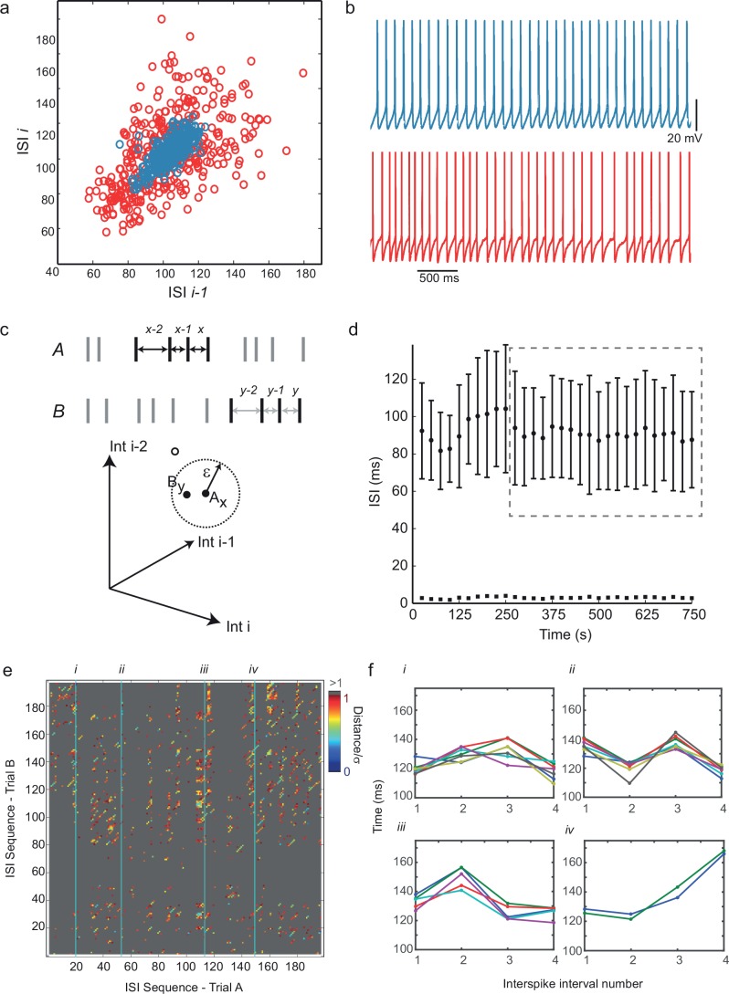
Figure 2. Predictability and nonlinearity of interspike interval sequences.

(a) Examples of two contrasting ISI return maps extracted from a regular-spiking cell (blue, mean frequency 9.67 Hz, CVISI = 0.075) and an irregular-spiking cell (red, mean frequency 9.65 Hz, CVISI = 0.207). (b) Segments of corresponding spike trains. (c) Principle of recurrence analysis. The dynamical state of the process is represented by vectors of consecutive ISIs, or embedding points. In this example, point Ax in a 3-dimensional embedding of an interspike interval sequence A (whose coordinates are ISIsx-2, x-1 and x) is similar to point By in interspike interval series B (top), because their distance is less than a threshold ε (bottom). (d) Selection of stationary sequences of stimulus trials for recurrence analysis. The mean ISI in each trial lasting 8 s, repeated at 25 s intervals, is plotted with its standard deviation (filled circles and error bars), and the standard error of the mean (filled squares). Sections of the time series were accepted as sufficiently stationary if the average trial-to-trial change in mean ISI was less than half the average standard error of the mean (e.g. region shown in dashed gray rectangle). (e) Example cross-recurrence plot between two consecutive stimulus trials, A and B, embedding dimension m = 4, ε = one standard deviation of the ISIs. Position (x,y) is colored according to the Euclidean distance between the length-4 ISI sequences at position x in A and y in B. Thus blue points reflect recurrence of very similar patterns. (f) Four examples of repeated patterns or 'motifs' of ISIs in sequence B corresponding to the patterns at positions (i)–(iv) in sequence A, as indicated in (e). See Figure 2—figure supplement 1 and Figure 2—source data 2 for recurrence plot quantification.

DOI: http://dx.doi.org/10.7554/eLife.16475.004

Figure 2—source data 1. Numerical values for Figure 2d.
DOI: 10.7554/eLife.16475.005
Figure 2—source data 2. Table showing details of recurrence plot analysis in ten cells.
Nonstationarity is the ratio of the average change in mean ISI in consecutive trials, divided by the standard error of the mean ISI. Time series with nonstationarity > 0.5 were rejected. In five of ten cells, both recurrence and determinism were significant (p< 0.05), only recurrence was significant in a further two cells, while in the three remaining cells, neither recurrence nor determinism were significant.
DOI: 10.7554/eLife.16475.006

Figure 2.

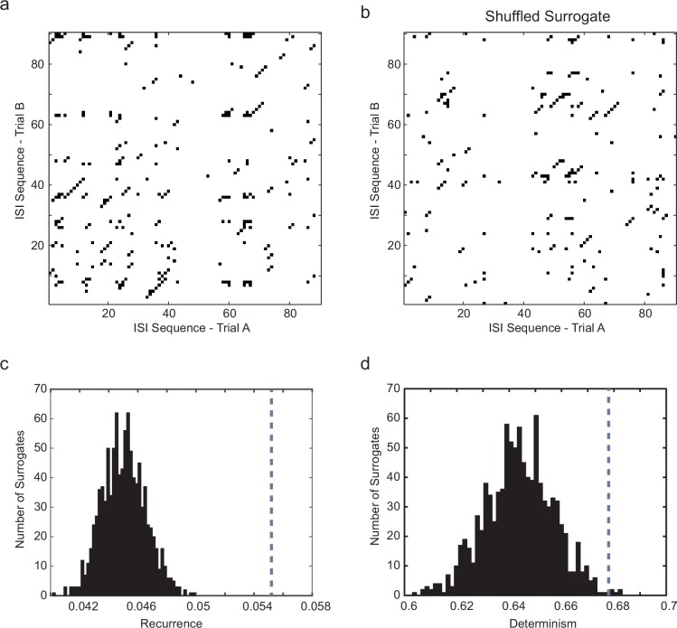
Figure 2—figure supplement 1. Significance testing of recurrence and determinism of interspike interval sequences.

Figure 2—figure supplement 1.

(a) Example cross-recurrence plot for the response to one 30 s current step trial against that of the subsequent trial. Threshold (ε) = σISI, embedding dimension = 4. Each point colored black denotes where sequences of 4 ISIs in each of the two trials were closer than ε to each other. (b) random shuffling of both sets of ISIs results in a loss of recurrence (proportion of black points in the matrix) and determinism (fraction of black points within diagonals of length 2 or greater. (c) Distribution of the recurrence values (each of which is the mean over 7 successive pairwise comparisons of consecutive 10 s trials during stationary firing) for 1000 shuffled surrogates (each ISI sequence in the CRP is randomly permuted), compared to the actual corresponding measured recurrence level (indicated by vertical dotted gray line) over the same set of trials. (d) the same for the determinism (fraction of recurrent points lying within diagonals of length ≥ 2). A z-test (Matlab ztest, right-tailed) confirms that both recurrence (p<7.52e-9) and determinism (p<0.023) are significant in this case.