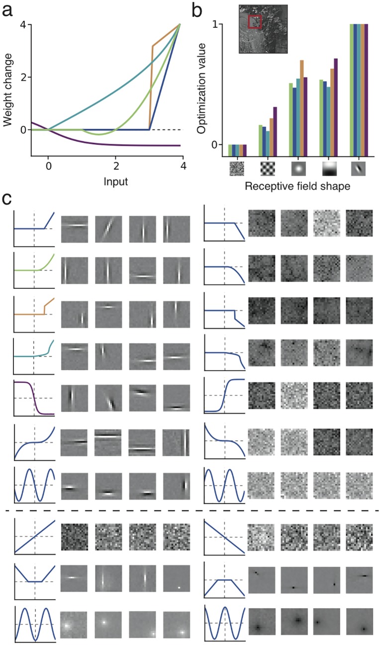
Fig 2. Simple cell development from natural images regardless of specific effective Hebbian nonlinearity.

(a) Effective nonlinearity of five common models (arbitrary units): quadratic rectifier (green, as in cortical and BCM models, θ₁ = 1., θ₂ = 2.), linear rectifier (dark blue, as in L₁ sparse coding or networks with linear STDP, θ = 3.), Cauchy sparse coding nonlinearity (light blue, λ = 3.), L₀ sparse coding nonlinearity (orange, λ = 3.), and negative sigmoid (purple, as in ICA models). (b) Relative optimization value 〈F(w^Tx)〉 for each of the five models in a, for different preselected features w, averaged over natural image patches x. Candidate features are represented as two-dimensional receptive fields. For all models, the optimum is achieved at the localized oriented receptive field. Inset: Example of natural image and image patch (red square) used as sensory input. (c) Receptive fields learned in four trials for ten effective Hebbian functions f (from top: the five functions considered above, u³, − sin(u), u, (|u| − 2)₊, − cos(u)) (left column), and their opposites − f (right column). The first seven functions (above the dashed line) lead to localized oriented filters, while a sign-flip leads to random patterns. Linear or symmetric functions are exceptions and do not develop oriented filters (bottom rows).