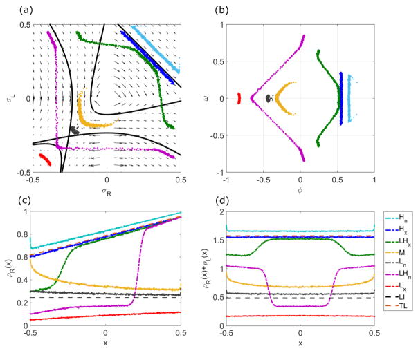
FIG. 6.

Examples of the nonlinear phases for low switching rate. (a) Trajectories in the σ_R-σ_L plane. (b) Trajectories in the ϕ-ω plane, where ϕ = σ_R + σ_L and ω = σ_R − σ_L, illustrating the local maxima and minima of the central density. (c) The density in lane R, ρ_R (x). The black dashed line (flat) indicates the LI in position space, and the brown dashed line (tilted) is the transition line in position space. (d) The total density as a function of position. The black dashed line indicates the LI (its value is 2ρ₀ since it is ρ_R + ρ_L) in position space, and the brown dashed line is the transition line in position space (its value is $-\frac{\gamma }{2S}+1$ since it is ρ_R + ρ_L). The boundary conditions are (α,1 − β) = (0.05,0.1) (red), (0.1,0.95) (purple), (0.3,0.4) (gray), (0.6,0.4) (yellow), (0.3,0.95) (green), (0.6,0.95) (blue), and (0.95,0.99) (cyan). The switching rate is 0.1 s⁻¹, the bulk motor concentration c = 200 nM, and the motor speed 5 μm s⁻¹; other parameters are the reference values of Table I. Arrows in (a) indicate the vector field, which has the mathematical form of Eqs. (12) and (13).