Figure 1.

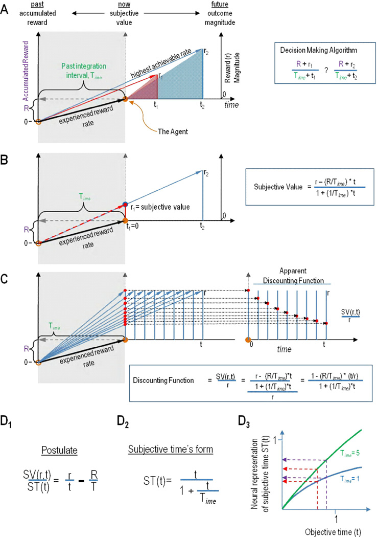
A) The TIMERR decision-making algorithm (right) can be depicted graphically (left) so as to visualize how offers of given reward sizes (r) and delays (t) are evaluated. An agent (filled orange circle), by looking into its past over an interval T_ime, assesses the rewards accumulated (R), thereby appreciating the reward rate experienced in the environment up to that moment. The local reward rates associated with current offers of future reward (slopes of red and blue offers) are then added to the experienced reward rate so as to calculate respective reward rates that could be achieved, were the agent to pursue an offer.

B) The TIMERR decision-making algorithm can be used to derive an expression for the subjective value of an offer, by equating an immediate offer of reward with a delayed offer of greater size but which yields the same achievable reward rate. By rearranging for subjective value, it is then appreciated that the opportunity cost of time (R/T_ime* t) is subtracted from a reward option (right inset). Graphically, the subjective value of a delayed reward is the y-intercept “now” in time of the line depicting the achievable reward rate were the agent to pursue that reward option (left).

C) The TIMERR decision-making algorithm can also be re-expressed as a temporal discounting function in terms of the fraction of an offer’s magnitude as a function of time (inset). The discounting function can be visualized by re-plotting the subjective value of a reward that is delayed through time at the offered reward’s respective delay (left). The resulting function is hyperbolic.

D) The form of subjective time under TIMERR. D₁) TIMERR postulates that the subjective reward rate of an offer should equal the difference between the local reward rate of an offer and the experienced reward rate. D₂) Subjective representation of time (ST(t)) is then found by replacing the subjective value of a delayed reward of magnitude r and delay t, SV(r,t), with its equation in B, and solving for ST(t). D₃) We hypothesize that the neural representation of time is ST(t) normalized by T_ime, as shown in the y-axis. This neural representation of subjective time yields a bounded, concave function from 0 (corresponding to zero delay) to 1 (corresponding to infinite delay). The smaller the past integration interval (T_ime), the more non-linear the neural representation of time (as visualized in D₃).