. 2016 Sep 26;5:e13451. doi: 10.7554/eLife.13451

Figure 3. During VWM retention, inter-areal CFS was both strenghtened and suppressed in harmonic structures.

(a) Fractions (K+) of inter-areal CFS connections that were significantly stronger during VWM maintenance than in the pre-stimulus baseline (Mean condition, Wilcoxon signed ranked test, < 0.05, corrected). K+ values (color scale) are shown for all studied pairs of 1:m ratios from 1:2 to 1:9 (x-axis) and lower frequencies from 3.3 to 45 Hz (y-axis) and represent data from an adjacency matrix for each frequency-pair. The grey line marks the boundary set by the highest investigated frequency (90 Hz). CFS of high-θ and high-α with their upper frequencies was increased for essentially all ratios. Right: The brown line indicates the harmonic consistency of CFS across low frequencies. The dashed line denotes the 95%-ile confidence limit. CFS of high-θ and high-α oscillations with their harmonics at higher frequencies is significantly consistent across ratios. (b) Fractions of inter-areal CFS connections (K-) that were suppressed below baseline levels during the retention period. Harmonic consistency (blue line) was estimated as in and shows that low-α consistent CFS was suppressed at all ratios.(c) Fractions of CFS connections that were significantly positively (K+) or (d) and negatively (K-) correlated with VWM load (Spearman Rank correlation test of CFS across the six VWM memory load conditions, < 0.05, corrected).

DOI: http://dx.doi.org/10.7554/eLife.13451.007

Figure 3.

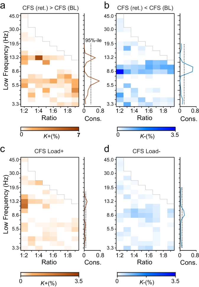
Figure 3—figure supplement 1. Workflow.

Figure 3—figure supplement 1.

This Figure provides a schematic overview of the analysis steps underlying the results shown in Figures 39. (a) Data pre-processing, see Materials and methods: Data pre-processing. (b) Filtering into 25 frequency bands with Morlet Wavelets (see Materials and methods: Filtering). (c) Preparation of forward and inverse operators (see Materials and methods: Preparation of forward and inverse operators). (d) Inverse transform to obtain external source data (Siebenhühner et al., 2016; see Materials and methods: Inverse transform and vertex collapsing) (e) Vertex collapsing onto a parcellation of 400 brain regions. (f) 1:1 and CF synchrony analysis (see Materials and methods: 1:1 and CF synchrony analysis) (g) Collapsing onto a courser parcellation of 148 brain regions (see Materials and methods: Group-level statistics). (h) Group-level statistics to obtain the Mean and Load effect (see Materials and methods: Group-level statistics) (i) Estimation of CFS & PAC consistency across ratios (see Materials and methods: Estimation of consistency across ratios). (j) Construction of summary graphs across ratios for θ and α consistent CFS (see Materials and methods: Construction of summary graphs across ratios). (k) Bundling of edges into hyperedges to better identify true interactions from signal mixing (see Materials and methods: Bundling of edges into hyperedges). (l) Assessment of interactions between functional brain subsystems of the Yeo parcellation (see Materials and methods: Assessing interactions within and between functional brain systems). (m) Correlation between networks of CFS and 1:1 phase synchrony (see Materials and methods: Correlation between networks of CFS and 1:1 phase synchrony). (n) Correlation of subjects’ individual network strength in CFS and PAC with their behavioural performance (see Materials and methods: Correlation of CFS and PAC with the behavioral performance).
Figure 3—figure supplement 2. Leave-one-out statistics and effect size thresholding corroborate the robustness of CFS observations.

Figure 3—figure supplement 2.

(a) Fractions (K+) of significant positive observations in the Mean condition (as in Figure 3 that survive thresholding with leave-one-out statistics. Here for the 12 subjects in our cohort, 12 leave-one-out cohorts of 11 subjects were created by leaving one subject out at a time. Each cohort was subjected to the same Mean condition group statistics and only those edges of the original findings (Figure 3a) were considered significant that were significant in every one of the 12 leave-one-out cohorts at the alpha level of p < 0.05. Preservation of a frequency-ratio pattern very similar to the original shows that the main findings are statistically robust and not attributable to any single subject in the cohort. (b) Fractions of significant positive observations in the Mean condition (as in Figure 3a) that also show an effect size > 0.9, which corresponds to statistical power of 0.8 or greater at N = 12. Preservation of a frequency-ratio pattern very similar to the original findings shows that the effects reported here are mostly of adequate size to be measured with the present number of subjects. (c) Fractions of edges remaining after both the leave-one-out (b) and effect size (c) thresholding. (d) Same as (a), but for the Load condition. (e) Same as (b) but for the Load condition where the effect size threshold was set to a correlation coefficient greater than 0.35. (f) As in (c), fractions of edges in original Load condition statistics that remain after combined leave-one-out (e) and effect size (f) masks.
Figure 3—figure supplement 3. Apparent signal-to-noise ratio (aSNR) in source space.

Figure 3—figure supplement 3.

aSNR was measured for each cortical parcel, time window, frequency band, and experimental condition as the ratio of the observed filtered signal amplitude and identically pre-processed and inverse transformed signal amplitude from empty-room MEG recordings. The figure shows Mean-condition aSNR estimates averaged across subjects and cortical parcels for the baseline (red) and the average of retention period (blue) time windows.
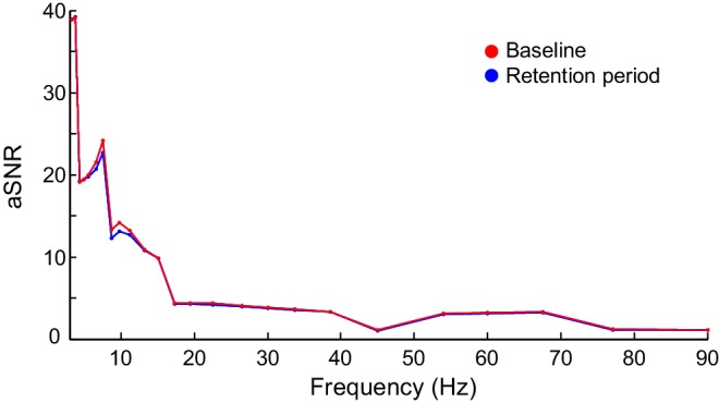
Figure 3—figure supplement 4. CFS PLV changes in the Mean condition are not attributable changes in the signal-to-noise ratio (SNR).

Figure 3—figure supplement 4.

Observed changes in CFS-PLV compared against changes in PLV predicted by the local changes in SNR from the baseline to the VWM retention period. Values are shown for the 200 largest observed PLV changes for representative frequency ratios where the largest group level effects were observed. The red line represents the ideal prediction of equal values between the observed and predicted PLV. Dots left to the red line thus represent edges for which the observed PLV is greater than predicted by event-related changes in SNR.
Figure 3—figure supplement 5. Observed PLV changes in the Load condition are not predicted by changes in SNR.

Figure 3—figure supplement 5.

The Load condition was approximated by the difference in CFS-PLV between Load 1 and Load 6 conditions. As in Figure 3—figure supplement 4, the observed changes in this CFS-PLV difference are compared with changes in PLV that are predicted from changes in SNR from the 1 object to 6 Object condition. Values are shown for the 200 largest observed PLV changes each for the frequency ratios shown in Figure 3—figure supplement 4.
Figure 3—figure supplement 6. Changes in PLV and amplitude are not correlated.

Figure 3—figure supplement 6.

(a) Variance in PLV changes that can be explained by amplitude changes in the Mean condition. Values r2∙sign(r) are shown only for ratio-frequency pairs that had > 0.1 % in the group analysis and showed a significant correlation between PLV and amplitude effects (r) in lowest or highest 2.5% of surrogate values, = 1000, uncorrected for multiple comparisons). (b) Same as (a), but for the Load condition. 
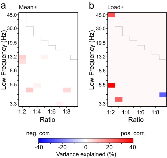
Figure 3—figure supplement 7. Cross-frequency (CF) amplitude-amplitude correlations do not have a low-frequency consistent harmonic structure.

Figure 3—figure supplement 7.

(a) Fractions of edges (K+) of inter-areal CF amplitude correlations that are significantly stronger during VWM retention period than in the baseline (Mean condition, as in Figure 3a). Unlike CFS, CF amplitude correlations did not show a harmonic pattern over low frequencies. (b) Fractions of significant edges of amplitude-amplitude correlations that were positively correlated with the VWM load (Load condition, as in Figure 3c).
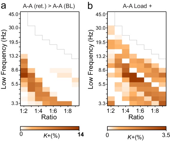
Figure 3—figure supplement 8. Connections with significant CFS are not co-localized with those exhibiting significant CF amplitude correlations.

Figure 3—figure supplement 8.

Fractions of edges, K, which were significant in (a) Mean- and (b) Load-conditions in both the CFS and CF-amplitude correlation analyses. Compared to the original networks (see Figure 3a,c and Figure 3—figure supplement 6) these very low K values show that there is little neuroanatomical co-localization in the networks of CFS and CF amplitude correlations.