Figure 6.

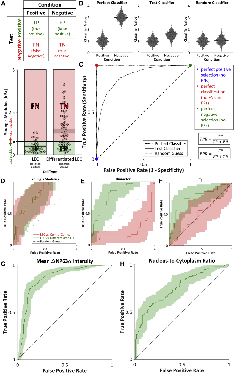
ROC curves. (A) For a binary classifier, the contingency table separates test subjects into TPs, FPs, FNs, and TNs. Young’s modulus was used to select for LECs (condition positive) and against differentiated LECs (condition negative). Cells below and above the threshold Young’s modulus (e) were considered to be test positive and test negative, respectively. (B) A perfect classifier would enable perfect discrimination between condition-positive and condition-negative cells (no FPs, no FNs), whereas a random classifier would enable no discrimination between condition-positive and condition-negative cells (TPs = FPs, TNs = FNs). In practice, the threshold value of a test classifier can be shifted to improve positive selection at the cost of reduced negative selection, or vice-versa. (C) ROC curves (black lines and D–H) were generated by calculating the TPR and FPR for all possible threshold values. The ROC curve for a test classifier (solid line) lies between the ROC curves for a perfect classifier (dotted line) and a random guess (dashed line). (D–H) ROC curves for the selection of LECs against either central cornea cells or differentiated LECs using the test positive conditions of a (D) low Young’s modulus; (E) low diameter; (F) low, slow viscoelastic time constant (τ₂); (G) high mean ΔNP63α intensity; or (H) high nucleus/cytoplasm ratio indicated that each parameter can be used to discern stemness. Shaded regions indicate 95% CI. To see this figure in color, go online.