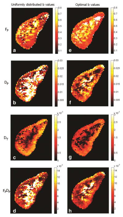
FIG. 3.

Biexponential parametric maps for a healthy kidney. Subplots (a–d): FP, DP, DT, FP × DP by using 10 uniformly distributed b values (rounded to the nearest b values available) [0, 100, 200, 250, 350, 400, 500, 600, 650]; subplots (e–h), by 10 optimal b values (rounded to the nearest b values available) [0, 50, 50, 50, 250, 250, 250, 750, 750, 750]. Maps obtained using the optimal b values have smoother texture and better rendering of renal cortex.
