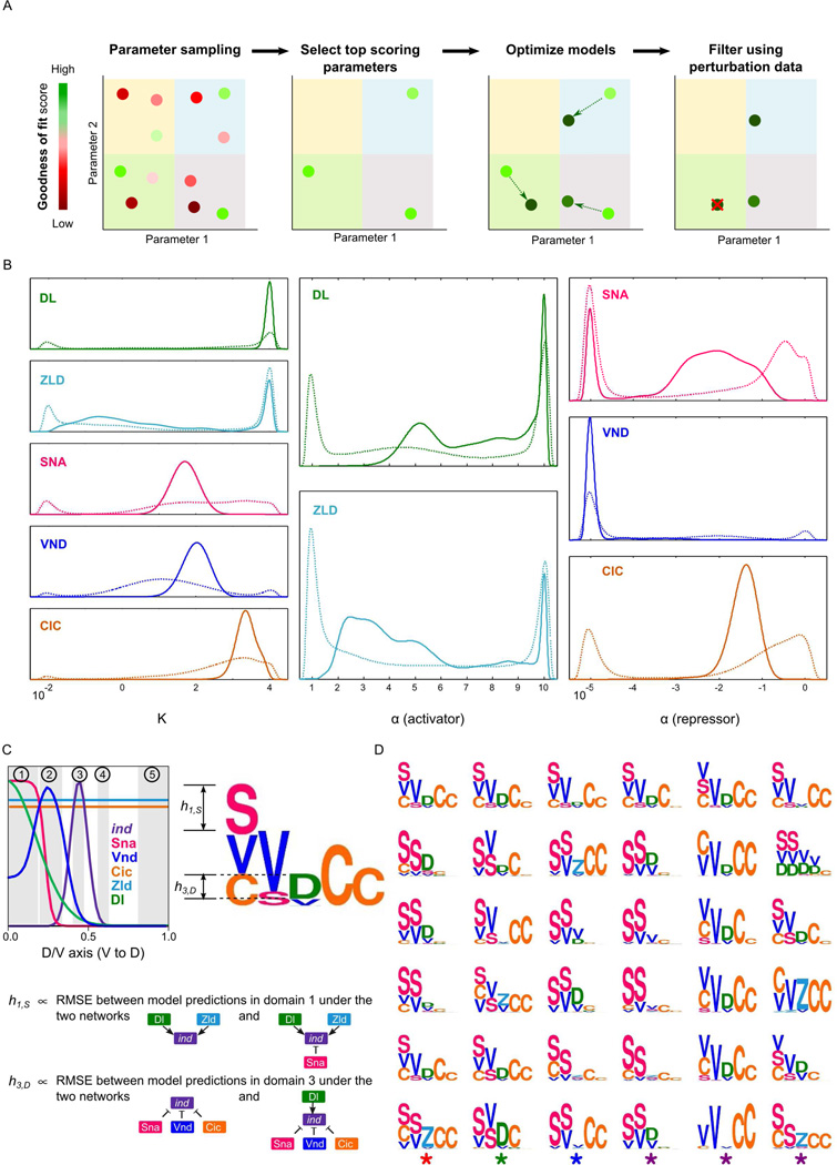
Figure 3.

Construction and visualization of model ensembles. (A) Left to right: sampling of parameter vectors, scoring, model optimization initiated from each parameter vector which scored above the threshold (the resulting set of optimized models is the “wild-type ensemble”), and filtering of wild type models according to their accuracy in predicting the effects of various perturbations. The remaining models (not crossed-out) constitute the “filtered ensemble”. (B) Marginal densities of parameters of the wild-type and the filtered ensemble models (dashed and solid lines, respectively). (C) The motif for a model shows how it utilizes each TF to regulate ind in five domains along D/V axis. Each domain corresponds either to the peak expression domain of ind (domain 3) or a TF (domains 1 and 2: peak expression domains of Sna and Vnd, respectively), or to a domain where the effect on ind expression is known for a specific site-mutagenesis experiment (domains 4 and 5: results known for Cic site mutagenesis). Columns in a motif correspond to domains, symbols denote the regulator TFs, and the height of a symbol in a column represents the contribution of that TF in the corresponding region: if a TF f is an activator then its height in a column represents the root-mean-squared-error (RMSE) between model-predicted ind expression profiles in the corresponding domain when there is no activator and when f is the only activator in the model. Similarly, the height of a repressor f is computed from the conditions when there is no repressor and when f is the only repressor in the model. (D) Representative motifs of the 36 clusters computed from the wild-type ensemble models.