Using Semi-Markov processes to study timeliness and tests used in the diagnostic evaluation of suspected breast cancer

Abstract

Diagnostic evaluation of suspected breast cancer due to abnormal screening mammography results is common, creates anxiety for women and is costly for the healthcare system. Timely evaluation with minimal use of additional diagnostic testing is key to minimizing anxiety and cost. In this paper we propose a Bayesian Semi-Markov model that allows for flexible, semi-parametric specification of the sojourn time distributions and apply our model to an investigation of the process of diagnostic evaluation with mammography, ultrasound and biopsy following an abnormal screening mammogram. We also investigate risk factors associated with the sojourn time between diagnostic tests. By utilizing Semi-Markov processes we expand on prior work which described the timing of the first test received by providing additional information such as the mean time to resolution and proportion of women with unresolved mammograms after 90 days for women requiring different sequences of tests in order to reach a definitive diagnosis. Overall, we found that older women were more likely to have unresolved positive mammograms after 90 days. Differences in the timing of imaging evaluation and biopsy were generally on the order of days and thus did not represent clinically important differences in diagnostic delay.

1 Introduction

Screening for breast cancer with mammography has been shown to reduce breast cancer morbidity and mortality [1–3]. However, abnormal results are common and must be followed-up with diagnostic evaluation through additional imaging and, in some cases, biopsy. As a result, diagnostic evaluation of abnormal mammography results is extremely costly, estimated at over $675 million per year in the US Medicare population alone [4]. Abnormal results also create anxiety for women [5]. Decreasing the number of tests required to reach a definitive diagnosis as well as the length of time between abnormal mammography findings and resolution of diagnostic evaluation is key to decreasing the burden on women and improving the efficiency of screening mammography.

Prior studies have evaluated the use of diagnostic imaging and biopsy following abnormal screening mammography results [6–9]. These studies have focused on descriptive characterization of the type and frequency of follow-up imaging received and the delay between receipt of abnormal results and follow-up with imaging or biopsy. By focusing on receipt of individual diagnostic tests, they have been unable to characterize the complete course of diagnostic evaluation including all imaging tests or biopsies received and the timing of the intervals between those tests. The process of evaluation with a series of imaging tests and biopsies can be characterized as a sequence of transitions among discrete states. This is similar to the conceptualization of many disease processes. For instance, diseases such as HIV may be described by transitions between an uninfected state, an infected pre-symptomatic state, a clinically detectable state, and death. Semi-Markov processes (SMP) provide a flexible approach to modeling processes characterized by repeated events and multiple failure types because they allow for flexible modeling of the distribution of the sojourn times. Although a few prior studies have made use of SMPs to describe biomedical processes (e.g., [10–12]), SMPs have generally seen limited use in this field. SMPs can also be useful in health services research where they can aid in understanding delays in receipt of medical care but to our knowledge SMPs have been used in only a few instances [13].

One of the major obstacles to broader application of these models is the increased complexity of estimation in the framework of Semi-Markov as compared to Markov models. Existing software implementations of SMPs have several limitations hampering their broad use in health applications. In biomedical and health services research, covariates are typically of high importance because the role of patient or disease characteristics associated with differences in transition probabilities or rates is often a key question. However, some existing software implementations do not allow for covariate dependence [14, 15]. Similarly, biomedical data sets typically consist of many subjects who are each observed to experience a small number of transitions. This is in contrast to other applications such as economics or meteorology where observations may consist of data for a single replicate observed through hundreds or thousands of transitions [14]. Finally, most existing software implementations of SMPs require parametric assumptions about the sojourn time distributions.

In this paper we explore the use of SMPs for characterizing the timeliness of diagnostic evaluation following an abnormal screening mammogram and the use of specific diagnostic imaging modalities and biopsy. SMPs can be used to estimate the sojourn time distribution between individual pairs of states but can also be used to obtain measures of clinical interest that describe the entire process more fully. For instance, we can describe the average length of time preceding a diagnostic evaluation of any kind; the proportion of women requiring a given sequence of tests to reach diagnostic resolution; the median time between tests for a given sequence of tests; or the proportion of women with unresolved abnormal mammograms after a fixed period of time given the sequence of diagnostic imaging experienced.

We propose a Bayesian SMP model that features a flexible specification of the sojourn time distributions and allows for estimation of covariate effects. We use our model to analyze the process of diagnostic evaluation following an abnormal screening mammogram. In Section 2 we provide some brief background on SMPs and describe our model and the estimation approach used in our implementation. In Section 3.1 we use simulation studies to demonstrate the performance of our estimation approach, and in Section 3.2 we study the diagnostic evaluation of abnormal mammography. We conclude with a discussion of the implications of this approach for research on multi-state models in health services research in Section 4.

2 Methods

2.1 Semi-Markov process

Let S = {1, 2, … s} represent a finite sequence of possible states that the process under study may take. We assume that for each subject we observe all states visited by the subject during the observation period and the exact time at which each subject enters and leaves each state. Let z_k represent the (k + 1)th state visited, with z₀ equal to the initial state and t_k the length of stay in the kth state. We define θ(i) ≐ P(z₀ = i) as the probability that the process begins in state i, θ(i, j) ≐ P(z_n = j|z_n−1 = i) as the transition probability from state i to state j, and F_ij(t_n) ≐ P(t_n < t|z_n−1 = i, z_n = j) as the cumulative distribution function for the sojourn times with corresponding probability density function f_ij(t_n). Further, we assume that conditional on z_n and z_n−1, the sojourn time is only a function of t_n, the elapsed time spent in the current state, and does not depend on the total length of time since initiation of the process. Thus, for a single subject observed to make m transitions, the likelihood takes the form

$$L(\mathit{\theta })=\left(\theta (z_0)\prod _{n=1}^{m-1}\theta (z_{n-1},z_n)f_{z_{n-1},z_n}(t_n)\right){(\theta (z_{m-1},z_m)f_{z_{m-1},z_m}(t_m))}^{1-\delta }{\left(\sum _{z\in S}\theta (z_{m-1},z)(1-F_{z_{m-1},z}(t_m))\right)}^{\delta },$$ (1)

where δ is an indicator that the observation is right censored. Right censoring arises if the period of observation ends prior to a subject entering an absorbing state. See Ouhbi and Limnios [16] for a discussion of likelihood construction for SMPs. Thus, in our formulation, all sojourn times are observed up until the last observation where the sojourn time may be right censored.

This basic model can be extended to allow for covariate dependence of either the sojourn time distributions or transition probabilities or both. However, we note that allowing for covariate dependence of both the sojourn time distributions and transition probabilities may lead to a model that is poorly identified. In what follows we incorporate covariates by specifying the modeling of the sojourn times accounting for covariate effects. We focus on the effect of covariates on the timing, rather than type, of transitions because we believe this is more applicable to the context of health services utilization studies. In this type of study, the type of procedure, and hence the transition probability, is likely to be determined by clinical characteristics. For instance, in the context of diagnostic evaluation of an abnormal mammogram certain types of lesions are best imaged by ultrasound while others are best imaged by mammography. However, the timing of follow-up and therefore the sojourn time may vary according to patient characteristics such as socio-economic status. Our models focus on understanding these patient risk factors that may lead to delays in receipt of recommended care.

2.2 Semi-parametric sojourn distributions

In some cases it may be unrealistic to assume that the functional form of the sojourn time distributions is known. To relax this assumption, we propose a semi-parametric approach to modeling the hazard functions for the sojourn times via discrete mixture models. Several authors have investigated estimation for survival models using discrete mixtures to model the baseline hazard [17–20]. These approaches focus on modeling baseline hazards using either discrete mixtures of Beta distributions [17, 18], triangular distributions [19], or B-splines [20]. As demonstrated by Cai et al. [20], finite mixture models based on mixtures of triangular distributions or Beta distributions are special cases of finite mixtures of B-splines. Specifically, the mixture of Beta distributions can be shown to be a special case of a mixture of B-splines with no interior knots. Here we focus on a finite mixture of Beta distributions because they are computationally tractable and flexible enough to accommodate all hazard function shapes expected to be encountered in realistic biomedical examples. Below we extend this work to the case of an SMP using mixtures of Beta functions for computational convenience.

Representing the density and distribution functions of the sojourn times in terms of the (baseline) hazard function, h_ij(t), and its corresponding cumulative hazard, H_ij(t), we can rewrite the likelihood in equation (1), accommodating covariate adjustment, as

$$\begin{array}{l}L(\mathit{\theta })=\theta (z_0)\left(\prod _{n=1}^{m-1}\theta (z_{n-1},z_n)h_{z_{n-1},z_n}(t_n)exp({\mathit{\beta }}_{z_{n-1},z_n}^T{\mathit{X}}_{z_{n-1},z_n})exp(-H_{z_{n-1},z_n}(t_n)exp({\mathit{\beta }}_{z_{n-1},z_n}^T{\mathit{X}}_{z_{n-1},z_n}))\right)\\ \times {\left(\theta (z_{m-1},z_m)h_{z_{m-1},z_m}(t_m)exp({\mathit{\beta }}_{z_{m-1},z_m}^T{\mathit{X}}_{z_{m-1},z_m})exp(-H_{z_{m-1},z_m}(t_m)exp({\mathit{\beta }}_{z_{m-1},z_m}^T{\mathit{X}}_{z_{m-1},z_m}))\right)}^{1-\delta }\\ \times {\left(\sum _{z\in S}\theta (z_{m-1},z)exp(-H_{z_{m-1},z}(t_m)exp({\mathit{\beta }}_{z_{m-1},z}^T{\mathit{X}}_{z_{m-1},z}))\right)}^{\delta },\end{array}$$ (2)

where X_i,j denotes the vector of covariates for transitions from i to j and β_i,j denotes the corresponding regression parameters. Note that in the above we utilize a proportional hazards formulation to account for the effects of covariates in the model. Thus, for the kth regression coefficient, $exp({\beta }_{i,j}^k)$ has the standard interpretation as the hazard ratio when comparing subjects that differ in the kth covariate by one-unit when all other covariates are held constant.

We modified the approach of Gelfand and Mallick [17] and Carlin and Hodges [18] to accommodate the multiple types of transitions inherent to the SMP as follows. Let J_ij(t) = a_ijH_ij(t)/(a_ijH_ij(t) + b_ij), where a_ij, b_ij > 0. This rescaling of H_ij creates a monotone function on (0, 1) that can be treated as a cumulative distribution function. We further assume that H_ij(t) = t, a simplifying assumption that corresponds to a linear rescaling of H_ij(t). We can then model J_ij(t) as a discrete mixture of cumulative distribution functions. Let Be(t|c, d) denote the Beta density with parameters c and d and IB(t|c, d) denote its corresponding cumulative distribution function. We model J_ij(·) as a mixture with

$$J_{ij}(t;{\mathit{w}}_{ij})=\sum _{l=1}^r{w}_{ij}^{l}IB(a_{ij}t/(a_{ij}t+b_{ij})\mid c_{ij}^l,d_{ij}^l),$$

where w_ij is a vector of weights with lth element $w_{ij}^l$ and ${\sum }_{l=1}^r{w}_{ij}^l=1$. This is motivated by the result of Diaconis [21] showing that any cumulative distribution function can be approximated arbitrarily well by a finite mixture of Beta cumulative distribution functions. We can use this to compute the corresponding cumulative hazard function, H_ij(t) = b_ijJ_ij(t; w_ij)/(a_ij(1−J_ij(t; w_ij))), and hazard function

$$h_{ij}(t)=b_{ij}\frac{\partial J_{ij}(t;{\mathit{w}}_{ij})}{\partial t}/(a_{ij}{(1-J_{ij}(t;{\mathit{w}}_{ij}))}^2),$$

with

$$\frac{\partial J_{ij}(t,{\mathit{w}}_{ij})}{\partial t}=a_{ij}{b}_{ij}/{(a_{ij}t+b_{ij})}^2\sum _{l=1}^r{w}_{ij}^{l}Be(a_{ij}t/(a_{ij}t+b_{ij})\mid c_{ij}^l,d_{ij}^l).$$

2.3 Bayesian estimation

Bayesian estimation has been used frequently for estimating the parameters of multi-state processes (e.g., [22–24]). Bayesian estimation is straightforward in this context given that the likelihood function is explicit. There are a number of advantages to using Bayesian estimation for SMPs. Because the number of parameters increases quickly as the number of states in the model increases, it is often the case that one or more types of transitions is infrequently observed. Under the Bayesian approach we can specify informative priors based on existing scientific information for these infrequently observed transitions, allowing for model estimation. Non-informative priors can still be used for more frequently observed transitions. An additional advantage is the ability to obtain estimates of the posterior predictive distribution for complex functionals of the model parameters. Under the Bayesian formulation, we require prior distributions for all model parameters, that is, θ(i), θ(i, j), β and w. Let η denote the collection of all model parameters. We assume a Dirichlet prior for the vector of initial state probabilities, (θ(1), …, θ(s)), and for each row of the matrix of transition probabilities, (θ(i, 1), … θ(i, s)). Likewise, we assume a Dirichlet prior for w. Finally, we assume Normal priors for regression coefficients.

Prior work indicated that arbitrary values of a and b perform equally well [17] and that a and b should be selected for computational convenience to ensure that observations occur throughout the entire range of J_ij(t; w_ij). Thus, the values of a and b that re-scale the cumulative hazard are fixed, and the same values are used for all transitions. We also assume fixed and known values for $c_{ij}^l$ and $d_{ij}^l$. Choices for these parameters determine the collection of Beta densities that will be components of the mixture. As recommended by previous work, we set $c_{ij}^l=\lambda l$ and $d_{ij}^l=\lambda (r+1-l)$ for all i and j, where λ determines how peaked the component densities will be [17]. In numerical examples presented below we assumed λ = 1.

Estimation is carried out via Markov Chain Monte Carlo (MCMC) with Metropolis-Hastings steps within Gibbs Sampling [25]. To address right censoring we consider a data-augmentation approach [26]. Thus, besides η we also estimate, within the MCMC procedure, the unobserved final transition for each right-censored observation. Sampling of an unobserved state is based on a multinomial full conditional distribution. Once the unobserved states are updated, the updating of the initial state probabilities and each row of the transition probability matrix follow from their corresponding Dirichlet full conditional distributions. Updating of the sojourn time parameters, both those describing the baseline hazard, as well as those describing the regression parameters, are updated via Metropolis-Hastings steps in two separate blocks: one for the regression parameters and another for the baseline hazard parameters (weights). We transform the weights using a logit transformation. Finally, in each block, we use multivariate normal proposal distributions.

2.4 Diagnostic evaluation of suspected breast cancer in the Breast Cancer Surveillance Consortium

We studied the process of diagnostic evaluation following an abnormal screening mammogram using data collected by five mammography registries in the National Cancer Institute-funded Breast Cancer Surveillance Consortium (BCSC) [27] (http://breastscreening.cancer.gov). These registries link information on women who receive a mammogram at a participating facility to regional cancer registries and pathology databases to determine breast cancer outcomes. Information on patient characteristics collected at the time of the mammogram included patient age, clinical history, and breast cancer risk factors.

Data come from women age 40–89 years with a screening mammogram at one of 15 BCSC mammography facilities within five of the BCSC regional mammography registries (Carolina Mammography Registry, Group Health Registry in Washington state, New Hampshire Mammography Network, San Francisco Mammography Registry, Vermont Breast Cancer Surveillance System) that provided information on follow-up mammography, ultrasound, and biopsy subsequent to a screening mammogram. All included women received a screening mammogram with an abnormal result, defined as a Breast Imaging Reporting and Data Systems (BI-RADS) [28] assessment of 0, 4, or 5 or an assessment of 3 accompanied by a recommendation for immediate evaluation, in 2005–2009. For women who received multiple positive screening exams during the study period, only the first was used. We included data for diagnostic evaluation with mammography, ultrasound, and biopsy beginning on the day after the positive screening mammogram and continuing for a period of 90 days.

The states in model of the process of diagnostic evaluation included a woman’s first instance of diagnostic mammography, diagnostic ultrasound, and fine needle aspiration or biopsy (for simplicity referred to subsequently as biopsy) after an abnormal screening mammogram. We created a combined state, “diagnostic mammogram and ultrasound,” which a woman entered once she had experienced exams of both types. A goal of our analysis was determining the time from receipt of an abnormal mammography result to diagnostic resolution either via a subsequent negative diagnostic imaging examination or a biopsy. We therefore divided states in the model into unresolved and resolved/terminal states. An imaging examination was considered to result in diagnostic resolution if it was negative (BI-RADS assessment of 1 or 2). We assumed that all biopsies that occurred within 90 days led to diagnostic resolution. The state space of the model is therefore S={1=screening mammogram; 2=diagnostic mammogram, unresolved; 3=diagnostic ultrasound, unresolved; 4=diagnostic mammogram + ultrasound, unresolved; 5=biopsy; 6=diagnostic mammogram, resolved; 7=diagnostic ultrasound, resolved; 8=diagnostic mammogram+ultrasound, resolved}. The potential transitions between states are depicted in Figure 1.

Figure 1.

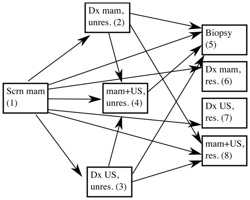
States and transitions in the model for diagnostic evaluation of an abnormal screening mammogram. The states are {1=screening mammogram; 2=diagnostic mammogram, unresolved; 3=diagnostic ultrasound, unresolved; 4=diagnostic mammogram + ultrasound, unresolved; 5=biopsy; 6=diagnostic mammogram, resolved; 7=diagnostic ultrasound, resolved; 8=diagnostic mammogram+ultrasound, resolved}. Scrn mam = screening mammogram, Dx mam = diagnostic mammogram, US = ultrasound.

We investigated patient characteristics potentially associated with variation in the use of diagnostic imaging and biopsy. Covariates of interest included BI-RADs breast density (categorized as non-dense (BI-RADs a and b) vs. dense (BI-RADs c and d)); age; and rural/urban status. We first used descriptive statistics to summarize transition probabilities and cumulative incidence functions (CIFs) for transition from each state. To describe the transitions between pairs of states, we calculated CIFs for transitions from each state with respect to time since state entry, using the R package cmprsk. To empirically investigate the shapes of the hazard functions, we plotted smoothed empirical hazard functions for the each of the transitions with respect to time, using a smoothing bandwidth of .3 months.

We modeled the diagnostic evaluation process using the semi-parametric Beta mixture model. We set a = 1 and b = 10, as these values yielded adequate mixing of the MCMC sampler, and informal experimentation with other values demonstrated that cumulative incidence estimates for sojourn times were insensitive to choice of these parameters. We compared model fit of models using exponential sojourn time distributions and using the semi-parametric mixture distribution with varying numbers of mixture components using the Bayesian Information Criterion (BIC). For the mixture model, we initially modeled the process using two or three component mixture distributions. However, to capture the steep slope of the CIF early in the follow-up period followed by a relatively flat hazard later in the follow-up period, such as that observed for transitions from state 4 to 5, we also investigated a model additing two additional mixture components, namely, Beta(2,32) and Beta(4,2).

We specified a Dirichlet prior with all parameters equal to 10 for the mixture weights of the sojourn distribution parameters for all transitions. Priors for log transformed covariate effects were independent Normal(μ = 0, σ² = 1) for all transitions, except for 3 to 4 and 3 to 8, which had small sample sizes in the data. Because these transitions were infrequently observed we did not attempt to estimate covariate effects on these transitions, specifying informative Normal(μ = 0, σ² = 10⁻⁷) priors for the corresponding regression parameters to effectively constrain them to be 0.

We ran the MCMC sampler for a total of 50,000 iterations, discarding the first 10,000. We used random walk multivariate normal distributions for the logit of the mixture weights in the sojourn distributions. We assessed mixing of the sampler via traceplots. We obtained 5 chains using different randomly chosen starting values, based on Normal(μ = 0, σ² = 0.5) distributions. To assess convergence of the sampler, we examined the posterior means from these 5 runs, and computed the Gelman and Rubin potential scale reduction factor [29]. We assumed that the chains had reached the equilibrium distribution if this statistic was less than 1.1. Our final estimates of the posterior densities combined the samples from each of the chains.

We sought posterior summaries of derived quantities in the model that described pairwise transitions as well as those summarizing the complete process of diagnostic evaluation. These quantities summarized time from the abnormal screening exam to the first diagnostic evaluation, time to diagnostic resolution, proportion of women with unresolved mammograms after 90 days, and transition times between states conditional on the specific pathway required to reach resolution. We investigated these quantities overall and conditional on covariates. Obtaining derived quantities involving transitions across multiple states requires integration over multiple pathways. We therefore estimated the posterior predictive distributions of these quantities by simulating sample trajectories of 10,000 observations for each posterior sample of model parameters and then computing the quantity of interest across the 10,000 observations.

3 Results

3.1 Simulation studies

We utilized simulation studies to assess the performance of the Bayesian estimation procedure. Specifically, our simulation studies are based on 100 replications where, for each scenario, we simulated data for N = 1000 subjects. Repeating the simulations 100 times allowed us to estimate parameters with Monte Carlo error of 0.02 or less. The maximum number of observations per subject was m = 10. We considered a four-state SMP that allowed for transitions between all pairs of states with no absorbing state. The transition probability matrix θ^T = {θ(i, j), i, j ∈ S} was

$$\mathit{\theta }=\left[\begin{array}{cccc}0.0& 0.6& 0.3& 0.1\\ 0.4& 0.0& 0.5& 0.1\\ 0.1& 0.5& 0.0& 0.4\\ 0.1& 0.2& 0.7& 0.0\end{array}\right]$$

and initial state probability vector was θ^I = {θ(i), i ∈ S} = (0.5, 0.3, 0.1, 0.1). We simulated the sojourn times between any pair of states under the semi–parametric sojourn distribution described previously in Section 2.2 using a = 1 and b = 20 and with two sets of weights to demonstrate two different shapes of the underlying hazard functions. Specifically, the hazard functions were specified using weights w_a = (0.693, 0.126, 0.181) or w_b = (0.164, 0.140, 0.695).

We evaluated our estimation method considering presence or absence of covariates, and presence or absence of censoring. In scenarios that utilized covariates we considered both a binary and a continuous covariate. The binary covariate was simulated from a Bernoulli distribution with mean 0.2. The continuous covariate was simulated from a Normal(0,1) distribution. Covariates were centered prior to carrying out estimation. We also investigated the effect of model misspecification by simulating data with these two covariates and then fitting the model with no covariates. In the scenario based on hazard function w_a with censoring, we applied administrative censoring at a maximum follow-up time of 5.5, which corresponds to 20–30% of the subjects being censored. Likewise, in the scenario based on hazard function with weights w_b with censoring, administrative censoring at a maximum follow-up time of 25 was applied, corresponding to 20–30% of the subjects being censored.

We first investigated relatively non-informative priors, a Dirichlet(1,1,1) for the weights and Normal(0,100) for the regression parameters. We then investigated sensitivity of results to use of more informative priors, Dirichlet(6,6,6) and Normal(0,0.5). We obtained a total of 10,000 posterior samples from our MCMC after a burn-in of 2500 initial iterations. We obtained posterior means, posterior variances and 95% posterior credible intervals for each model parameter. We evaluated the posterior estimates for bias, root mean squared error (RMSE) and coverage of the credible intervals across 100 replications.

Estimates for the weights for our semi-parametric hazard function reflected the shape of the true underlying hazard function. Supporting Web Material Figures 1 and 2 provide true and estimated hazard functions based on these weights. Hazard functions were generally more precisely estimated early in the observation period with variance in estimated hazard functions increasing over time. Table 1 shows simulation results averaged over all transitions. In simulations using weights w_a coverage probabilities for w₂ and w₃ were inflated above the nominal 95% level. This may reflect the fact that these parameters are only weakly identifiable in this setting. Across all scenarios, regression parameters were estimated well with relatively little bias. However, bias in these parameter estimates was larger under scenarios with censoring. Coverage probabilities for regression parameters were also below 95% in the presence of censoring. These results suggest that for sample sizes and prior distributions similar to those used in the simulations, the prior strength may have notably influenced posterior estimates for some parameters, especially in cases where some observations are censored. Results presented separately for each transition are provided in Supporting Web Material Tables 1–4. In general, results for individual weights and regression parameters were highly similar across transition types. There did not appear to be any systematic differences in performance of the estimation approach across transition types.

Table 1.

Simulation results for MCMC estimation for the semi-parametric SMP. Scenarios vary with respect to the underlying hazard function (hz), number of covariates (cov) and whether administrative censoring was applied. The table reports the posterior mean (Estimate), posterior standard deviation (SD), root mean squared error (RMSE), and coverage probabilities of the 95% posterior credible intervals averaged over all transitions and across 100 replications of each scenario.

Scenario	Parameter	True values	No censoring				With censoring
			Estimate	SD	RMSE	Coverage	Estimate	SD	RMSE	Coverage
1: hz wa, no cov	w1	0.693	0.685	0.031	0.032	0.95	0.684	0.033	0.034	0.94
	w2	0.126	0.161	0.074	0.082	1	0.161	0.074	0.082	1
	w3	0.181	0.154	0.07	0.075	1	0.155	0.071	0.075	1
2: hz wa, 2 covs	w1	0.693	0.684	0.034	0.035	0.95	0.684	0.038	0.039	0.95
	w2	0.126	0.162	0.074	0.082	1	0.159	0.075	0.082	1
	w3	0.181	0.153	0.07	0.075	1	0.157	0.072	0.076	1
	β1	0.2	0.208	0.128	0.128	0.96	0.243	0.134	0.141	0.94
	β2	0.5	0.502	0.052	0.052	0.94	0.459	0.061	0.073	0.85
3: hz wb, no cov	w1	0.164	0.161	0.012	0.012	0.96	0.16	0.013	0.014	0.95
	w2	0.14	0.175	0.063	0.072	0.94	0.18	0.069	0.08	0.95
	w3	0.695	0.664	0.055	0.063	0.94	0.66	0.061	0.071	0.95
4: hz wb, 2 covs	w1	0.164	0.161	0.013	0.013	0.96	0.162	0.014	0.014	0.96
	w2	0.14	0.178	0.064	0.074	0.95	0.173	0.069	0.076	0.96
	w3	0.695	0.662	0.057	0.066	0.95	0.666	0.062	0.069	0.96
	β1	0.2	0.19	0.129	0.129	0.94	0.221	0.137	0.139	0.95
	β2	0.5	0.512	0.055	0.056	0.94	0.462	0.063	0.074	0.86

Finally, we investigated the sensitivity of results to model misspecification and choice of priors. Using the set of true weights, w_a, we simulated data incorporating covariate effects and then fit a model excluding covariates. We found that failure to include covariates had relatively minimal effects on parameter estimates for the weights (Supporting Web Material Table 5). Bias in parameter estimates was similar in magnitude to that observed under correct model specification. When more informative priors were used for weights (Dirichlet(6,6,6)) and regression parameters (Normal(0,0.5)), posterior means were observed to deviate towards the prior means more substantially while regression parameters exhibited minimal effect (Supporting Web Material Table 6). As stronger priors are introduced, results are anticipated to be increasingly influenced by prior specification, but for a data set of the size investigated in simulations, we found results to be relatively insensitive to priors of the strength investigated.

3.2 Diagnostic evaluation after abnormal mammography

A total of 40,046 positive mammograms met study inclusion criteria. Characteristics of the sample are described in Table 2. The mean age was 55.6 years. Overall, the sample lived predominantly in urban areas (90%). Non-dense breasts were found in 40% of women, and dense breasts in 60%. Breast density and rural/urban status each were missing for about 8% of women. Subsequent analyses are reported on the complete cases, leading to a final sample size of 33,179 women. Table 3 shows the observed counts of transitions between successive states in the model based on this complete case sample.

Table 2.

Characteristics of women in the BCSC with positive screening mammograms included in the study of diagnostic evaluation.

	N	%	N missing
Age group
<50	15491	38.7
50–59	12806	32.0
≥60	11749	29.3
BI-RADS breast density			3455
Non-dense (BI-RADS a and b)	14776	40.4
Dense (BI-RADS c and d)	21815	59.6
Rurality			3524
Rural	3617	9.9
Urban	32905	90.1

Table 3.

Transition probabilities for multi-state model for diagnostic evaluation after abnormal mammography. Rows represent starting states and columns represent ending states. States are defined as 1=screening mammogram; 2=diagnostic mammogram, unresolved; 3=diagnostic ultrasound, unresolved; 4=diagnostic mammogram + ultrasound, unresolved; 5=biopsy; 6=diagnostic mammogram, resolved; 7=diagnostic ultrasound, resolved; 8=diagnostic mammogram+ultrasound, resolved. Scrn mam = screening mammogram, Dx mam = diagnostic mammogram, US = ultrasound

Ending state
Starting state	1	2	3	4	5	6	7	8	No transition	Total
Scrn mam (1)	0	2272 (6.9%)	265 (.80%)	3137 (9.5%)	84 (.25%)	13534 (40.8%)	1117 (3.4%)	10952 (33.0%)	1818 (5.5%)	33179
Dx mam, unres (2)	0	0	0	106 (4.7%)	1463 (64.4%)	0	0	445 (19.6%)	258 (11.4%)	2272
US, unres (3)	0	0	0	14 (5.3%)	151 (57.0%)	0	0	13 (4.9%)	87 (32.8%)	265
Mam+US, unres (4)	0	0	0	0	2639 (81.0%)	0	0	0	618 (19.0%)	3257

Time to resolution is summarized in Figure 2, which shows the CIFs for resolution of the abnormal screening examination overall and by the final type of diagnostic exam. The median time to resolution was 11 days (IQR [7,20]). Within 30 days of the screening examination, 84% were resolved and within 90 days, 91.9% were resolved. Biopsy was required to reach resolution in 13.1% of cases; 41.1% were resolved via diagnostic mammography; 34.5% via diagnostic mammography and ultrasound; and 3.3% using only ultrasound. Estimated smoothed hazards for each transition are provided in Supporting Web Materials Figure 3. Of the models compared, the SMP with sojourn distributions based on the five component mixture of Betas minimized the BIC (Table 4). Samples from the posterior predictive distribution for the five component mixture model also corresponded well with the empirical CIFs indicating adequate model fit.

Figure 2.

Cumulative incidence of time to resolution overall and by last diagnostic state. Black lines represent the empirical estimates, and colored lines are for 500 samples from the posterior distribution of the CIFs.

Table 4.

Bayesian Information Criterion (BIC) for four alternative Semi-Markov process models for the process of diagnostic evaluation of suspected breast cancer.

Sojourn distribution	Number of parameters	BIC
Exponential	24	115596.1
Two component mixture	24	118222.8
Three component mixture	38	113515.6
Five component mixture	66	107290.3

The posterior distributions of the adjusted covariate effects for each of the sojourn distributions are summarized in Figure 3. (Numerical estimates are available in Supporting Web Materials Table 7.) The age effects represent the unit change in log hazard for each 10 year age increment. Many of the covariate estimates for all three parameters include zero. The covariate estimates for age indicate modestly lower hazard rates for older ages for transitions from an abnormal screening exam to diagnostic mammography ((1,2), (1,6), (1,8)) and to biopsy from diagnostic mammography with and without ultrasound ((2,5), (4,5)). Dense breasts were associated with lower hazards for some transitions from screening mammography ((1,2), (1,6)) and diagnostic mammography ((2,4), (2,8)). Living in an urban location was associated with higher hazards for transitions from diagnostic mammography with or without ultrasound to biopsy((2,5), (4,5)).

Figure 3.

Summary of posterior distributions of covariate effects for conditional hazards, adjusting for age, breast density, and urban/rural status. Points represent the median value and intervals, the 2.5th and 97.5th quantiles. The states are {1=screening mammogram; 2=diagnostic mammogram, unresolved; 3=diagnostic ultrasound, unresolved; 4=diagnostic mammogram + ultrasound, unresolved; 5=biopsy; 6=diagnostic mammogram, resolved; 7=diagnostic ultrasound, resolved; 8=diagnostic mammogram+ultrasound, resolved}.

Covariate-specific posterior summaries of the mean time to resolution and proportion of women with unresolved mammograms both overall, and by last occupied state, are shown in Figure 4. Overall, time to resolution was longer for abnormal exams requiring biopsy. Times to resolution for exams resolved by only a single imaging modality (either diagnostic mammography or ultrasound) were similar with those requiring both mammography and ultrasound to reach resolution requiring slightly more time. Women with unresolved abnormal results after 90 days most often had received only the initial screening mammogram with no subsequent imaging follow-up. In general, older women experienced slightly longer times to resolution and were more likely to have unresolved mammograms after 90 days.

Figure 4.

Summary of posterior distribution for the mean time to resolution (A) and proportion of unresolved mammograms at 90 days (B) by the last visited state across covariate groups. Estimates were obtained via simulation of 10,000 samples for each MCMC parameter sample. Intervals represent 2.5th and 97.5th quantiles of the posterior distributions.

Finally, we investigated the process of diagnostic evaluation by summarizing transitions across multiple states. Figure 5 illustrates median transition times between states for women with dense and non-dense breasts. The proportion of women following each pathway was similar regardless of breast density. Transitions to unresolved diagnostic mammogram (state 2) and biopsy (state 5) occurred slightly later and to unresolved ultrasound (state 3) occurred slightly earlier for women with dense breasts compared to those with non-dense breasts. Transitions to resolved imaging states (6, 7, 8) occurred after similar elapsed times for the two groups.

Figure 5.

Median transition times by breast density among urban women, age 55, for each pathway to a resolved mammogram within 90 days of an abnormal screening mammogram. Times are based on posterior predictive distributions obtained via 10,000 simulations from the model. Percentages represent the proportion of women taking each pathway to a resolved mammogram within 90 days. States are defined as 1=screening mammogram; 2=diagnostic mammogram, unresolved; 3=diagnostic ultrasound, unresolved; 4=diagnostic mammogram + ultrasound, unresolved; 5=biopsy; 6=diagnostic mammogram, resolved; 7=diagnostic ultrasound, resolved; 8=diagnostic mammogram+ultrasound, resolved

4 Discussion

We developed a Bayesian SMP under continuous observation. Adopting this approach can provide additional insight into the dynamics of biomedical and health services applications beyond what is possible when states are considered individually. Our estimation approach is computationally feasible even for large data sets and extends the tools available for analyzing SMPs beyond what is currently available. By applying this methodology in the context of health services utilization we were able to examine patterns of care for patients with suspected breast cancer in greater depth than has been possible in previous studies in which individual types of diagnostic examinations were examined separately. The proposed approach has broad applicability to studies of the timing of health services utilization, an area in which SMPs have seen limited previous use.

In an application of our estimation approach to the diagnostic evaluation of suspected breast cancer, we found that most cases were resolved after use of diagnostic mammography or ultrasound, with a minority requiring both imaging modalities or biopsy. This finding is similar to previous studies, [6, 7, 9]. However, by developing a multi-state model for this process we were able to evaluate additional characteristics of the process of potential clinical interest. We found that older women were more likely to have unresolved abnormal results after 90 days and tended to take longer to reach diagnostic resolution. However, differences between groups were small. Similar to prior analyses [9], we found that differences in time to resolution across patient sub-groups were generally on the order of days. This magnitude of delay is not clinically significant and thus provides reassurance that among the patient characteristics investigated, sub-groups of women do not experience diagnostic delays that could lead to adverse outcomes.

In addition to investigating the length of time to diagnostic resolution, the SMP representation of the diagnostic process allowed us to investigate possible covariate effects on the timing of states visited. In the context of health services utilization, this is important for identifying patient sub-groups who may experience protracted diagnostic evaluation and who might benefit from use of alternative evaluation methods. We found that breast density, which has received much attention as a risk factor for breast cancer and also is associated with poorer mammography performance, had little effect on the timing of transitions. Small delays in transitions to diagnostic mammography were observed for women with dense breasts. However, these were on the order of a week or less. This provides reassurance that women with dense breasts are receiving appropriate management.

Multi-state models are infrequently used in studies of health services utilization likely because of the strong parametric assumptions required by Markov models and the difficulty of conducting estimation for more flexible SMPs. A few prior studies of receipt of health care services have used SMPs (e.g., [13, 30]). However, these have generally been limited by reliance on parametric assumptions about the sojourn time distributions. Several software packages exist for estimation of SMPs. However, they lack capabilities for dealing with key features of health services data including the presence of covariates and large data sets with relatively few observations per individuals. The Bayesian estimation approach described here provides the ability to handle both of these characteristics, potentially broadening the available tool kit for working with these types of data.

One challenge in using the semi-parametric hazard function specification is in choosing the number of components to include in the mixture distribution. In our analysis of data on diagnostic evaluation of suspected breast cancer, we investigated mixtures including 2–5 components and selected the 5 component model based on descriptive investigation of the empirical hazards and comparison of BIC. Similarly, the choice of whether to use a semi-parametric specification for the hazards versus a parametric distribution or whether a Markov process is adequate or a Semi-Markov process is required can also be evaluated using BIC. Goodness of fit statistics for multi-state models have been proposed by Saint-Pierre et al. [31] and can also be used for these purposes.

Strengths of our approach include its ability to accommodate processes with arbitrary numbers of states and patterns of allowed transition among states. We have also developed a semi-parametric specification for sojourn times. A particular strength of the Bayesian estimation approach is the ability to obtain posterior samples for complex functionals of the model, corresponding to quantities of clinical interest. These are typically challenging to obtain analytically but can be obtained relatively easily via posterior (predictive) simulation under the Bayesian framework.

Like all estimation methods for multi-state models, parameter estimates related to infrequently observed transitions may be unstable. While such transition types can be incorporated into analyses, investigators should take into consideration that informative priors may be needed and that the resulting inference will likely be sensitive to choice of the prior distributions.

A specific limitation of our investigation of diagnostic evaluation of suspected breast cancer is the possibility of missing data on follow-up examinations. Because women may receive care outside of the BCSC, some follow-up examinations may not have been captured. We attempted to mitigate the effect of incomplete capture by limiting our analysis to 15 facilities where previous comparisons of BCSC follow-up records and Medicare claims for subsequent diagnostic evaluation verified that the majority of follow-up was captured [9]. However, it is likely that some women did receive care at outside facilities. This would upwardly bias estimates of the proportion of women whose positive mammogram remained unresolved at 90 days and estimates of time to resolution.

In conclusion, this work provides an alternative method for estimation of parameters of biomedical and health services processes that can be conceptualized as multi-state models. Future work will extend this framework to accommodate processes that are observed intermittently, giving rise to panel data.

References

- 1.Humphrey LL, Helfand M, Chan BK, Woolf SH. Breast cancer screening: A summary of the evidence for the US Preventive Services Task Force. Annals of Internal Medicine. 2002;137(5):347–360. doi: 10.7326/0003-4819-137-5_part_1-200209030-00012. [DOI] [PubMed] [Google Scholar]
- 2.Nelson HD, Tyne K, Naik A, Bougatsos C, Chan BK, Humphrey L. Screening for breast cancer: An update for the US Preventive Services Task Force. Annals of Internal Medicine. 2009;151(10):727–737. doi: 10.1059/0003-4819-151-10-200911170-00009. [DOI] [PMC free article] [PubMed] [Google Scholar]
- 3.Smith RA, Duffy SW, Gabe R, Tabar L, Yen AM, Chen TH. The randomized trials of breast cancer screening: What have we learned? Radiologic Clinics of North America. 2004;42(5):793–806. doi: 10.1016/j.rcl.2004.06.014. [DOI] [PubMed] [Google Scholar]
- 4.Lee DW, Stang PE, Goldberg GA, Haberman M. Resource use and cost of diagnostic workup of women with suspected breast cancer. The Breast Journal. 2009;15(1):85–92. doi: 10.1111/j.1524-4741.2008.00675.x. [DOI] [PubMed] [Google Scholar]
- 5.Brett J, Bankhead C, Henderson B, Watson E, Austoker J. The psychological impact of mammographic screening. A systematic review. Psycho-Oncology. 2005;14(11):917–938. doi: 10.1002/pon.904. [DOI] [PubMed] [Google Scholar]
- 6.Carney P, Abraham L, Miglioretti D, Yabroff K, Sickles E, Buist D, Kasales C, Geller B, Rosenberg R, Dignan M, et al. Factors associated with imaging and procedural events used to detect breast cancer after screening mammography. American Journal of Roentgenology. 2007;188(2):385–392. doi: 10.2214/AJR.05.1718. [DOI] [PubMed] [Google Scholar]
- 7.Carney P, Kasales C, Tosteson A, Weiss J, Goodrich M, Poplack S, Wells W, Titus-Ernstoff L. Likelihood of additional work-up among women undergoing routine screening mammography: The impact of age, breast density, and hormone therapy use. Preventive Medicine. 2004;39(1):48–55. doi: 10.1016/j.ypmed.2004.02.025. [DOI] [PubMed] [Google Scholar]
- 8.Welch HG, Fisher ES. Diagnostic testing following screening mammography in the elderly. Journal of the National Cancer Institute. 1998;90(18):1389–1392. doi: 10.1093/jnci/90.18.1389. [DOI] [PubMed] [Google Scholar]
- 9.Hubbard R, Zhu W, Horblyuk R, Karliner L, Sprague B, Henderson L, Lee D, Onega T, Buist D, Sweet A. Diagnostic imaging and biopsy pathways following abnormal screen-film and digital screening mammography. Breast Cancer Research and Treatment. 2013;138(3):879–887. doi: 10.1007/s10549-013-2466-5. [DOI] [PMC free article] [PubMed] [Google Scholar]
- 10.Kang M, Lagakos S. Statistical methods for panel data from a semi–Markov process, with application to HPV. Biostatistics. 2007;8(2):252–264. doi: 10.1093/biostatistics/kxl006. [DOI] [PubMed] [Google Scholar]
- 11.Titman AC, Sharples LD. Semi-Markov models with phase-type sojourn distributions. Biometrics. 2010;66(3):742–752. doi: 10.1111/j.1541-0420.2009.01339.x. [DOI] [PubMed] [Google Scholar]
- 12.Kapetanakis V, Matthews FE, van den Hout A. A semi-Markov model for stroke with piecewise-constant hazards in the presence of left, right and interval censoring. Statistics in Medicine. 2013;32(4):697–713. doi: 10.1002/sim.5534. [DOI] [PMC free article] [PubMed] [Google Scholar]
- 13.Cao Q. The application of continuous-time Semi-Markov models in health economic decision making: A case study in heart failure disease management. The 36th Annual Meeting of the Society for Medical Decision Making; Society for Medical Decision Making; 2014. [DOI] [PubMed] [Google Scholar]
- 14.Bulla J, Bulla I, Nenadić O. HSMM—An R package for analyzing hidden semi-Markov models. Computational Statistics & Data Analysis. 2010;54(3):611–619. [Google Scholar]
- 15.O’Connell J, Højsgaard S. Hidden semi markov models for multiple observation sequences: The mhsmm package for R. Journal of Statistical Software. 2011;39(4):1–22. [Google Scholar]
- 16.Ouhbi B, Limnios N. Nonparametric estimation for semi-markov processes based on its hazard rate functions. Statistical Inference for Stochastic Processes. 1999;2(2):151–173. [Google Scholar]
- 17.Gelfand A, Mallick B. Bayesian analysis of proportional hazards models built from monotone functions. Biometrics. 1995;51(3):843–852. [PubMed] [Google Scholar]
- 18.Carlin B, Hodges J. Hierarchical proportional hazards regression models for highly stratified data. Biometrics. 1999;55(4):1162–1170. doi: 10.1111/j.0006-341x.1999.01162.x. [DOI] [PubMed] [Google Scholar]
- 19.Perron F, Mengersen K. Bayesian nonparametric modeling using mixtures of triangular distributions. Biometrics. 2001;57(2):518–528. doi: 10.1111/j.0006-341x.2001.00518.x. [DOI] [PubMed] [Google Scholar]
- 20.Cai B, Meyer R. Bayesian semiparametric modeling of survival data based on mixtures of B-spline distributions. Computational Statistics & Data Analysis. 2011;55(3):1260–1272. [Google Scholar]
- 21.Diaconis P, Ylvisaker D. Quantifying Prior Opinion, Bayesian Statistics. Vol. 2. North Holland; Amsterdam: 1985. [Google Scholar]
- 22.Pan SL, Wu HM, Yen AMF, Chen THH. A Markov regression random-effects model for remission of functional disability in patients following a first stroke: A Bayesian approach. Statistics in Medicine. 2007;26(29):5335–5353. doi: 10.1002/sim.2999. [DOI] [PubMed] [Google Scholar]
- 23.Wu GHM, Chang SH, Chen THH. A Bayesian random-effects Markov model for tumor progression in women with a family history of breast cancer. Biometrics. 2008;64(4):1231–1237. doi: 10.1111/j.1541-0420.2007.00979.x. [DOI] [PubMed] [Google Scholar]
- 24.van den Hout A, Matthews FE. Estimating dementia-free life expectancy for Parkinson’s patients using Bayesian inference and microsimulation. Biostatistics. 2009;10(4):729–743. doi: 10.1093/biostatistics/kxp027. [DOI] [PMC free article] [PubMed] [Google Scholar]
- 25.Gamerman D, Lopes H. Markov Chain Monte Carlo: Stochastic simulation for Bayesian inference. Vol. 2. Chapman & Hall; New York: 2006. [Google Scholar]
- 26.Tanner MA, Wong WH. The calculation of posterior distributions by data augmentation. Journal of the American Statistical Association. 1987;82(398):528–540. [Google Scholar]
- 27.Ballard-Barbash R, Taplin S, Yankaskas B, Ernster V, Rosenberg R, Carney P, Barlow W, Geller B, Kerlikowske K, Edwards B, et al. Breast Cancer Surveillance Consortium: A national mammography screening and outcomes database. American Journal of Roentgenology. 1997;169:1001– 1008. doi: 10.2214/ajr.169.4.9308451. [DOI] [PubMed] [Google Scholar]
- 28.D’Orsi C, Sickles E, Mendelson E, Morris E. ACR BI-RADS Atlas, Breast Imaging Reporting and Data System. American College of Radiology; Reston, VA: 2013. [Google Scholar]
- 29.Gelman A, Rubin DB. Inference from iterative simulation using multiple sequences. Statistical Science. 1992;7(4):457–472. [Google Scholar]
- 30.Crystal S, Lo Sasso AT, Sambamoorthi U. Incidence and duration of hospitalizations among persons with AIDS: An event history approach. Health Services Research. 1999;33(6):1611–38. [PMC free article] [PubMed] [Google Scholar]
- 31.Saint-Pierre P, Combescure C, Daures J, Godard P. The analysis of asthma control under a Markov assumption with use of covariates. Statistics in Medicine. 2003;22(24):3755–3770. doi: 10.1002/sim.1680. [DOI] [PubMed] [Google Scholar]
Associated Data
This section collects any data citations, data availability statements, or supplementary materials included in this article.