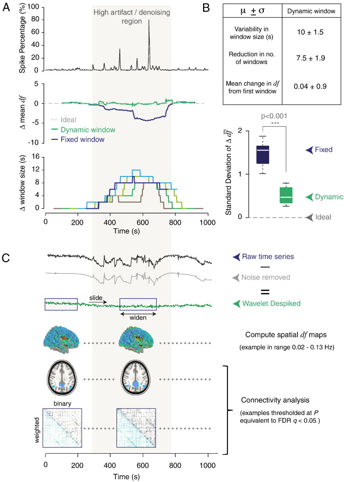
Fig. 7.

Application of the df method to time-windowed analysis.

(A) Upper panel shows the spike percentage (indicating the level of wavelet despiking required at each time point) for an example subject from cohort 3 showing high artifact levels in the middle of the run. The middle panel shows the mean (across voxels) change in total within-window df, from the first window. The blue line represents the fixed window method where a sliding window of length 200 s was used. The green line represents the same for the dynamic window approach. In this case, the window length was dynamically increased (minimum window size of 200 s) in low df regions in order to minimize window-to-window variation in df. Points plotted indicate the middle of each window. The lower panel shows the change in window size through time using the dynamic window approach, for window lengths of 100, 200, 300, 400 and 500 s. Points plotted indicate the middle of each window.

(B) The table describes the properties of the set of dynamic windows calculated for a range of minimum window lengths between 100 and 500 s. Boxplots show the standard deviation of the change in df from the first frame of data (e.g. of the trace shown in the middle of panel A), for a range of different (minimum) window lengths.

(C) Example of how the dynamic window approach can be used to generate windowed spatial df maps, which can then be used for functional connectivity or graph analyses, and statistically thresholded as described in Fig. 2, Fig. 4, Fig. 6.