Parenchymal Airspace Profiling: Sensitive Quantification and Characterization of Lung Structure Evaluating Parenchymal Destruction

Abstract

Lung morphometry was introduced over 50 years ago to provide quantitative evaluation of the lung structure. The existing parameters, such as mean linear intercept and destructive index, suffer from simplistic data interpretation and a subjective data acquisition process. To overcome these existing shortcomings, parenchymal airspace profiling (PAP) was developed to provide a more detailed and unbiased quantitative method. Following the standard protocols of fixation, embedding, and sectioning, lung micrographs were: (1) marked with nonparenchymal area, preprocessed, and binarized under the researcher’s supervision; (2) analyzed with a statistical learning method, Gaussian mixture model, to provide an unbiased categorization of parenchymal airspace compartments, corresponding to a single alveolus, alveolar sac, and ductal/destructive airspace; and (3) further quantified into morphometric parameters, including reference volume, alveolar count, and ductal/destructive fraction (DF) based on stereological principles. PAP was performed on hematoxylin and eosin–stained lung sections from mice and rabbits. Unbiased categorization revealed differences in alveolar size among several mouse strains (NZW/LacJ<AKR/J<A/J<C57BL/6J) and across species (mouse<rabbit). Further quantification indicates that parenchymal destruction, modeled in mouse lungs with 1-month smoke exposure, resulted in decreased alveolar count, increased DF, but no significant differences in mean linear intercept. DF also provides a robust measurement that is not biased by processing artifacts, magnification, or reference volume, which are common limitations in human lung biopsies or data obtained from different laboratories. PAP is a novel approach to lung morphometry that offers more detailed characterization of the lung structure, sensitivity, and robustness than presently used methods for evaluating parenchymal destruction.

Clinical Relevance

The method described in this study integrates statistical learning and human knowledge for unbiased characterization and accurate quantification of parenchymal airspace compartments. The methodology greatly improves the efficiency and strengthens the understanding of lung parenchymal structure, which will benefit studies examining developmental and pathological changes in the lung.

For over 50 years, investigators have used lung morphometry based on several stereological principals to detect differences in lung structure to characterize various lung conditions and evaluate animal models of lung diseases (1–4). Although in recent years there are new morphometric approaches that use computed topography, such as Vasilescu’s volumetric imaging technique to construct a three-dimensional (3D) acinar structure (5) and Scott’s nondestructive imaging of fixed and embedded tissue (6), there are no new user-friendly methods to evaluate lung pathology. In the field of lung research, particularly in animal models, computed topography is still limited by accessibility and image resolution, whereas the formalin-fixed, paraffin-embedded, and hematoxylin and eosin (H&E)–stained lung sections are easily generated; therefore, a new methodology based on H&E sections would be generally applicable.

The conventional manual stereology methods have been instrumental in identifying lung structure abnormalities in disease models, but are highly laborious (1, 7). One of the most widely used parameters is the mean linear intercept (MLI), also known as cord length, dating back to the 1950s (8, 9), achieved by adding gridlines and performing manual counting of a number of intercepts passing through a line. Although this method provides a scientific parameter with a unit of length, this method is easily biased by errors in scaling, differences in the degree of inflation, and tissue shrinkage during tissue collection and processing (1). Furthermore, even separate batches of experiments from the same laboratory may not be comparable, due to these variations, not to mention varying results generated between different laboratories. Another parameter particularly helpful for quantifying parenchymal destruction is the destructive index (DI), originally described in 1985 (10). The DI method uses 50 equally distributed dots overlaid on top of each image, and each dot is labeled as either a normal area (N) or an area of destruction (D) by a pathologist. The DI is calculated as the percentage value of D#/(D# + N#), where “#” is the number of D or N. Careful examination of 50 dots per image by a researcher is even more labor intensive than the MLI method, possibly one of the reasons that the DI is not widely used. More importantly, the subjectivity in differentiating the normal versus destructive area further amplifies the interobserver variations and results in lower reproducibility and comparability between laboratories. Despite the limitations, the DI method is still in use, due to its improved sensitivity in detecting mild emphysema compared with the method of MLI (11, 12).

The inefficient nature of traditional lung morphometry has further limitations. Because a tremendous amount of time is needed to complete the task, only a small fraction of the whole tissue can be analyzed. To avoid introducing bias in the sampling process, randomization becomes an essential step, but, in the meantime, the randomization process is difficult to document and affects the reproducibility of the results. Further attempts to shorten the processing time by using multiple observers would inevitably inflate the interobserver variation.

There has been some improvement in taking a computational approach for lung morphometric analysis. Sallon and colleagues (13) used ticks and closed area to provide quantitative evaluation of the pathophysiology of the developing and mature lungs. The closed area is an excellent indicator for lung development, but the tick counting can be more complicated, as it involves a specific algorithm written in MATLAB (MathWorks, Natick, MA), and has a much slower processing speed.

In the present article, we extend the general computational approach with additional, well accepted statistical learning methods on the area values of numerous airspaces to perform an unbiased characterization and accurate quantification of parenchymal airspace compartments. We also demonstrate the improved sensitivity and robustness of the parenchymal airspace profiling (PAP) compared with the traditional methods.

Materials and Methods

Animals

All animal studies were performed with the approval of the Institutional Animal Care and Use Committee of Columbia University. Male A/J, AKR/J, C57BL/6J, NZW/LacJ mice at 10 weeks of age were purchased from the Jackson Laboratory (Bar Harbor, ME). Female New Zealand white rabbits (weight, 1.3–1.8 kg) were obtained from Harlan Laboratories (Indianapolis, IN) and Charles River Laboratories (Wilmington, MA).

Cigarette Smoke Exposure

Mice were acclimated to the animal facility for at least 48 hours before use. After this, animals underwent smoke exposure in a TE-10 Teague Smoking Apparatus (Teague Enterprises, Woodland, CA) with 3R4F Reference Cigarettes (University of Kentucky, Lexington, KY). Total particulate matter was maintained at 100–150 mg/m³ as measured by an aerosol monitor DustTrak II 8,530 (TSI, Shoreview, MN) and confirmed by gravimetric analysis. Mice underwent smoke exposure 5 h/d, 5 d/wk for 1 month.

Tissue Preparation

Both mouse and rabbit lungs were pressure inflated (25 cm H₂O) with 10% formalin. The entire left lung from the mouse and four major lobes (left anterior/posterior and right anterior/posterior lobes) from the rabbits were then embedded in paraffin and step sectioned (5 μm in thickness) every 200 μm and H&E stained. MLI was calculated as previously described (14, 15).

Image Acquisition

Either one scanned image from Leica SCN400 (Leica Microsystems CMS GmbH, Wetzlar, Germany) was acquired, or more than 25 randomly sampled images under the Nikon Eclipse E400 (Nikon, Tokyo, Japan), were acquired for each slide. Whole slide scans were cropped and downsampled to 4–10× equivalent images before performing PAP. The magnification between 4× and 10× provided adequate resolving power for alveolar structure and sufficient coverage of the ductal/ destructive area if each individual view was captured under a microscope. The final pixel scale was 1 μm/px under the 10× objective for mice and 2.5 μm/px under the 4× objective for rabbits. The images were then organized into this folder structure: ∼\Group\Individual\Slide\Image.

Image Processing

The image preprocessing pipeline (16), which relies on computer vision modules, such as OpenCV (opencv.org; C/C++/Java/Python), AForge.NET (aforgenet.com; C#), and Image Processing Toolbox (MATLAB; MathWorks), has the following components: (1) preprocessing (exclude non-parenchyma areas by color and adjust the color/sharpness, etc.); and (2) binarization (apply a global threshold for the whole-slide scans or an adaptive thresholding method [17] for individual images taken under a microscope with noticeable vignetting to distinguish the tissue from airspaces). These processing steps and parameters were fine tuned by trained researchers. After binarization, data on all airspaces enclosed by lung septal tissue were retrieved with feature extraction operations from the previously mentioned modules, such as SimpleBlobDetector (OpenCV), BlobCounter (AForge.NET), and regionprops (Image Processing Toolbox).

Reference Volume Calculation

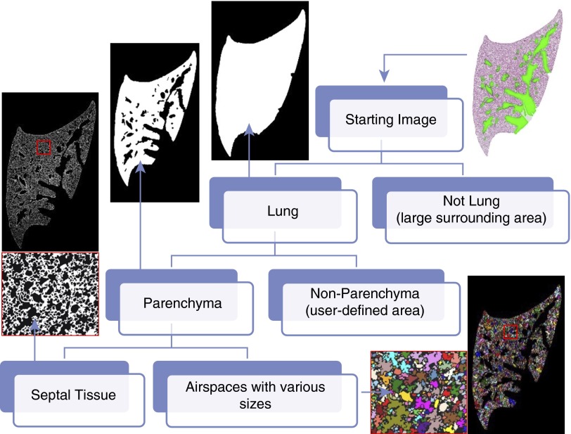
The raw pixel–based unit (px²) of the area was converted into actual area values (e.g., μm²), according to the pixel scale and resize ratio. As shown in Figure 1, automated computer processing and researcher supervision together yielded an accurate estimation of the lung area and parenchymal area per section. According to Cavalieri’s principle, V = ΣA_i × h, the area in each section can be used to estimate the reference volume. The lung area was estimated by excluding extra-large airspace (>10⁶ μm²) surrounding the lung section, and the parenchyma was estimated by further excluding colored nonparenchyma (Figure 1).

Figure 1.

Scheme of parenchymal airspace profiling (PAP). A hematoxylin and eosin–stained mouse lung section can be stratified into the areas of the lung, the parenchyma, the septal tissue, and the enclosed airspaces (randomly colored), with computer vision and researcher supervision. The reference volume can be estimated from the reference area of each section according to Cavalieri's principle. The area value of each airspace can be extracted for downstream categorization and quantification. Lung micrographs were processed from a whole slide scan (10× objective) of a mouse left lung.

Airspace Categorization

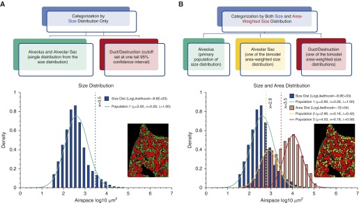
Area values (μm²) of numerous airspaces from each slide or individuals were log10 transformed to form a normal size distribution. Size distribution alone identified a predominate subpopulation of alveoli in the form of single alveolus (“a”) and alveolar sac (“s”), which derives to a ductal/destructive threshold (DT; based on upper 95% confidence interval) that separates the alveoli from the significantly larger ductal/destructive airspaces (“d”) (Figure 2A). With sufficient sampling (>1,000) of large airspaces, we further factored in each airspace’s area (μm²) to form an area-weighted size distribution by simple expansion or resampling algorithms (see Figure E1 in the online supplement). As the area-weighted size distribution displays a bimodal distribution, we characterized the two subpopulations with a Gaussian mixture model and expectation maximization algorithm (18, 19). Because the separation between the two subpopulations was consistent with DT based on size distribution alone (Figure 2B), and the smaller subpopulation was a few times larger than the alveolar size, these two were categorized as alveolar sacs (“s”) and ductal/destruction region (“d”).

Figure 2.

Categorization of parenchymal airspace compartments. (A) Single-distribution categorization (used only when limited large airspaces were sampled in the case of human biopsies or micrographs with a small field of view). Size distribution alone identifies a predominant population consisting of numerous alveoli. The distinction of normal and enlarged airspaces (alveolar duct or area of destruction) was made by upper 95% confidence interval (blue vertical line). (B) Double-distribution categorization (generally preferred method). In addition, area-weighted size distribution identifies two more subpopulations of airspaces, corresponding to alveolar sacs, and ductal/destructive airspaces. The data on all three subpopulations (μ, mean; σ, variance; λ, proportion) lead to the identification of two thresholds in between, represented by yellow and red vertical lines. Color-coded lung micrographs were processed from a whole slide scan (10× objective) of a mouse left lung.

Airspace Quantification

Categorization in two (as|d) or three (a|s|d) airspace compartments by single- or double-distribution methods allowed further quantification of each airspace compartment in parameters, such as N_A, B_A, and A_A, (number, boundary, and area per unit parenchyma area, respectively) (Table 1). Based on the fundamental principles of stereology (Table E1), these 2D parameters, especially for the single alveolus subpopulation, can have 3D interpretations, including N_V, S_V, and V_V.

Table 1.

Definition of Terms in Parenchymal Airspace Profiling

Term	Description
Nonparenchyma	Conducting airways and vessels.
Septal tissue	The thin structures that define the walls of the alveoli and the alveolar ducts.
Airspaces	Airspaces enclosed by septal tissue, based on the image-processing method.
Alveoli	Airspaces (1) that make up the majority of the airspaces, including alveolar sacs when performing single-distribution categorization; and (2) that make up the majority of airspaces and smaller than the size of alveolar sac when performing double-distribution categorization.
Ductal/destructive threshold	The threshold: (1) defined by upper 95% confidence interval for alveolar size when performing single-distribution categorization; or (2) defined as the size between the two subpopulations (alveolar sacs and ductal/destructive airspaces) in area-weighted size distribution. In practice, either of the two methods provides the consistent threshold value (Figure 3B).
Alveolar sac	Airspaces defined by the smaller one of the subpopulations in area-weighted size distribution when performing double-distribution categorization. As a subcategory of alveoli, each airspace is larger than a single alveolus but smaller than a ductal/destructive airspace.
Ductal/destructive airspaces	Airspaces defined by the larger one of the subpopulations in area-weighted size distribution when performing double-distribution categorization. Each airspace represents an alveolar duct or an area of destruction.
Size (A)	Sum of pixels within each airspace (only for a single airspace or as a group average), which was further converted to area (μm2) as a parameter.
Area (A)	Sum of pixels within each airspace or multiple airspaces under a particular category, which was further converted to area (μm2) as a parameter.
Count (N, NA), number density (NV)	Number of airspaces under a particular category, which was further converted to count per unit area (#/mm2) as a parameter and may be interpreted as number density in three dimensions with formulae in Table E1.
Boundary (B, BA), surface area per unit volume (SV)	Sum of pixels on the edge (eight-way connectivity) of each airspace or airspaces under a particular category, which was further converted to boundary per parenchymal area (μm/μm2) as a parameter and may be interpreted as surface area per unit volume with formulae in Table E1.
Fraction (%, AA, VV)	Area percentage of airspaces under a particular category to the lung parenchyma (μm2/μm2), which can be directly interpreted as volume fraction, according to formulae in Table E1.

Terminology used in the article for the development of parenchymal airspace profiling, in light of several previous publications (1–4).

Results

The Size Parameters Based on Unbiased Categorization Revealed Baseline Differences across Different Species, Even between Different Strains of Mice

According to the area data on thousands of airspaces, unbiased categorization by both size- and area-weighted size distribution identified three distinct subpopulations of airspaces corresponding to a single alveolus (“a,” small, colored green), an alveolar sac (“s,” medium, colored yellow), and an alveolar duct or an area of parenchymal destruction (“d,” large, colored red).

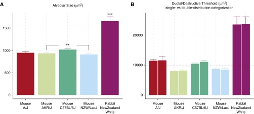
As shown in Figure 3A, the alveolar size from the smallest to the largest is as follows (presented as mean ± SEM): NZW/LacJ mouse, 907.57 ± 20.04 μm²; AKR/J mouse, 935.18 ± 18.14 μm²; A/J mouse, 947.74 ± 24.92 μm²; C57BL/6J mouse, 1,019.32 ± 19.65 μm²; New Zealand white rabbit, 1,659.52 ± 97.19 μm². As expected, the rabbit exhibited a significantly (P < 0.001) larger alveolar size than all of the mouse strains. Among the four mouse strains examined, the C57BL/6J strain exhibits significantly larger alveolar size than the AKR/J and NZW/LacJ (P < 0.01) strains.

Figure 3.

Either of the categorization methods generates accurate quantification of single alveolar size and consistent estimation of ductal/destructive threshold (DT). (A) Baseline alveolar size differences across different species and mouse strains. Alveolar size of the rabbits are significantly larger than any of the mouse strains (P < 0.001), and different mouse strains also exhibit baseline differences (P < 0.01 for C57BL/6J versus AKR/J and C57BL/6J versus NZW/LacJ). (B) Both single- and double-distribution categorization methods generated comparable DT values (A/J, P = 0.8973; C57BL/6J, P = 0.16; NZW/LacJ, P = 0.7623; AKR/J, P = 0.2809; rabbit, P = 0.8869). Data are presented as mean ± SEM. **P < 0.01; ***P < 0.001.

With sufficient sampling of small and large airspaces, there is no discrepancy between DT estimated by single-distribution (upper 95% confidence interval) or double-distribution categorization (between two subpopulations in area-weighted size distribution). Student’s t test between DT_1-dist and DT_2-dist was performed for all mouse strains and rabbits: A/J, P = 0.8973; C57BL/6J, P = 0.16; NZW/LacJ, P = 0.7623; AKR/J, P = 0.2809; and P = 0.8869 for New Zealand white rabbit. Either categorization approach provided a clear and consistent distinction between the alveoli and ductal/destructive airspaces (paired bars, Figure 3B).

The DT calculated with unbiased categorization followed a similar trend compared with the alveolar size, with A/J as the only exception. Although the A/J strain has a similar alveolar size as AKR/J and NZW/LacJ, the A/J lung exhibits significantly increased DT (P < 0.001, A/J versus AKR/J, A/J versus NZW/LacJ), which suggests that the alveolar ducts in A/J mice are larger than in the other strains (Figure 3B).

Further Quantification of Each Airspace Compartment Indicated That Parenchymal Destruction Is Primarily Reflected by Decreased Alveolar Counts and Increased Ductal/Destructive Fraction

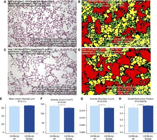
Two lung images, either healthy or emphysematous (Figures 4A and 4C), were processed through unbiased categorization and quantification (Figures 4B and 4D). In addition to coloring airspaces by their specific categorization, a list of parameters was calculated (Table 1, Figures 4E–4G). Among them, the most significantly affected parameters are alveolar count (↓AC; 1/mm², P = 0.04), alveolar boundary (↓AB; 1/μm, P = 0.019), and ductal/destructive fraction (↑DF; %; P = 0.00079). Compared with MLI (↑MLI, μm, P = 0.11), which did not reach the level of statistical significance, DF is more sensitive at detecting mild emphysema in C57BL/6J mice exposed to cigarette smoke for 1 month (Figure 4).

Figure 4.

Comparison of mean linear intercept (MLI) and parameters quantified with PAP. (A–D) Healthy (A) and emphysematous (C) mouse lungs were subjected to double-distribution categorization, color coding, and quantification (B and D). Three distinct subpopulations of airspaces corresponding to single alveolus, alveolar sac, and ductal/destructive airspace were colored green, yellow, and red, respectively. (E–H) Parameters generated from PAP, such as alveolar count (AC), alveolar boundary (AB), and ductal/destructive fraction (DF), exhibited improved sensitivity compared with MLI. Between smoke- and air-exposed mice: MLI, P = 0.11 (E); AC, P = 0.04 (F); AB, P = 0.019 (G); DF, P = 0.00079 (H). Data are presented as mean ± SEM. *P < 0.05; ***P < 0.001.

In Addition to Improved Sensitivity, DF Is Also More Robust in the Evaluation of Parenchymal Destruction Than MLI

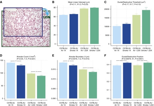
We artificially introduced scaling artifacts and bias on the scale factor by up-sampling all lung images to 125% while entering the original pixel scale (1 μm/px). As a result, this process produced biases in all parameters that refer to the actual dimension. MLI (μm, 1D) was increased by 1.2-fold. Alveolar count (1/mm², 1/2D) was decreased by 1.4-fold. AB (1/μm, 1/1D) was decreased by 1.2-fold. Only the dimensionless parameters, such as AF, SF, and DF, remained unbiased and, in particular, DF still showed significant differences between air- and smoke-exposed mice (Figure 5).

Figure 5.

Use of DF as a sensitive and robust assessment of parenchymal destruction. To test how well each parameter can withstand differences in scale factor and scaling artifacts, the original images were up-sampled to 125% while using the original pixel scale (A). After the process, most parameters, except for DF, were biased and showed less significant differences between smoke- and air-exposed mice. DF remained unbiased, because DT generated from unbiased categorization adapted to the differences in scale factor. Between smoke- and air-exposed mice after 125% magnification: MLI, ↑1.2-fold, P = 0.23 (B); DT, ↑1.7-fold, P = 0.13 (C); AC, ↓1.4-fold, P = 0.021 (D); AB, ↓1.2-fold, P = 0.015 (E); DF, no change, P = 0.0051 (F). Data are presented as mean ± SEM. *P < 0.05; **P < 0.01; ***P < 0.001.

Discussion

The method described here combines basic computer vision functionalities, well accepted statistical learning methods, and researcher supervision to offer optimal compatibility and reproducibility to quantify morphometric changes in lung structure. For optimal performance and responsive graphical user interface, a Windows desktop application implementing this method was developed, and is available at http://www.ruixiao85.net/home/download.

Point and intercept counting on a gridline system has been instrumental as a classical approach to measuring lung morphometry. As most lung micrographs are now digitized, pixels retain all the information for each sample. With an adequate amount of user supervision, computational approaches that innately perform analyses down to a single-pixel basis are more efficient and accurate than the traditional gridline-counting approach.

The area parameter, which represents the number of pixels located within the area of interest, represents the most basic estimation of each airspace, and can be interpreted into volume parameters in 3D. The boundary of each airspace can be a good alternative, as it can be interpreted into the 3D surface area (Table E1). Although the boundary is potentially inaccurate, with different degrees of magnification (higher magnification may show more jagged edges and result in overestimation) and different algorithms (four-way versus eight-way connectivity), the estimation of boundary is rather consistent before and after up-sampling to 125% (Figure 5). An expected 1.2-fold decrease and negligible differences in P value (P = 0.019 to P = 0.015) was found for AB (1/μm). Therefore, boundary estimated with computational approaches, although less ideal than the area, can still be a valid parameter and a good alternative to MLI derived from the traditional gridline-counting methods.

Although the computational approach is more efficient, researcher supervision and intervention is still essential to ensure that the automated process is adequately performed. Because the parenchymal versus nonparenchymal area of the lung cannot be easily distinguished, a user-defined area with contrasting color appears to be the proper approach that uses the efficiency of computers and allows for researcher oversight. For a designed experiment, the quick estimation of reference areas from step sections will enable efficient and accurate estimation of the reference volume of lung or parenchyma.

Both MLI and DI, as calculated by the traditional methods, increase during the process of parenchymal destruction. Because the MLI values are sensitive to scaling artifacts and differences in scale factor, variance within each group will inevitably interfere with the changes due to parenchymal destruction, and render the pathological changes less detectable or less significant (Figure 4E). The differences in scale factor, in a broader sense, include different degrees of magnification, inflation, and tissue shrinkage, because all of these processes uniformly influence the size of all airspaces, which will result in a global shift in the airspace sizes. Since the DT was dynamically calculated by statistical learning methods, it will adapt and shift accordingly (Figure 5C), and therefore continue to provide unbiased categorization and estimation of DF. The added robustness and comparability are helpful for various laboratory conditions: (1) different batches of experiments, researchers, and laboratories may result in different fixation, embedding, and section conditions; and (2) captured digital images of the lung may not be properly labeled for the exact magnification or pixel scale.

Although, in theory, DI is as sensitive and robust as DF, the subjective and laborious nature of the DI method has prevented the method from being widely used. There are only a handful of studies that use the DI, despite the fact that this method was introduced over 30 years ago. Compared with DI, DF manages to remove subjectiveness, with gains in processing efficiency.

In addition to offering a more sensitive and robust measurement of parenchymal destruction, the size categorization provides an excellent tool to measure the baseline dimensions of airspace compartments. As shown in Figure 3, PAP distinguishes the minor alveolar size differences among different strains of mice, and indicates that A/J mice at baseline generally have larger alveolar ducts.

The distinction between the healthy region of the lung that forms the refined segmentations to allow more effective gas exchange, and the unhealthy region where larger airspaces limit efficient gas exchange, is made by the unbiased statistical learning algorithm, but how the result is to be interpreted must be based on specific scientific questions. During the process of parenchymal destruction (e.g., induced by cigarette smoke), the “D” in the DF should be interpreted as “destructive” rather than “ductal” compared with the healthy controls. On the other hand, when comparing the baseline differences during the lung development process or among different normal populations, “D” should be interpreted as “ductal” because the alveolar duct is an integral part of the lung parenchyma in the normal state.

Forming the 3D structure is the ultimate goal to completely studying lung morphometry; however, the massive amount of data and difficulties in presenting 3D structure on a 2D surface are still the main obstacles. To achieve the same resolution of more than one pixel per micrometer (or ≤1 μm/px) under the microscope, a small piece of the lung that is 1 cm³ in size will take more than 10¹² pixels and occupy greater than 1 TB of hard drive space. Furthermore, the technologies for displaying and publishing 3D structural results are still under development. This method, as a first step, is focused on the data gathered from 2D sections and interpreted as 2D or 3D parameters with proper transformation (Table E1) under basic stereological principals.

In conclusion, PAP is a novel approach to lung morphometric analysis that offers detailed characterization of the lung structure and improved sensitivity and robustness compared with traditional methods for evaluating parenchymal destruction.

References

- 1.Hsia CC, Hyde DM, Ochs M, Weibel ER ATS/ERS Joint Task Force on Quantitative Assessment of Lung Structure. An official research policy statement of the American Thoracic Society/European Respiratory Society: standards for quantitative assessment of lung structure. Am J Respir Crit Care Med. 2010;181:394–418. doi: 10.1164/rccm.200809-1522ST. [DOI] [PMC free article] [PubMed] [Google Scholar]
- 2.Weibel ER. A retrospective of lung morphometry: from 1963 to present. Am J Physiol Lung Cell Mol Physiol. 2013;305:L405–L408. doi: 10.1152/ajplung.00169.2013. [DOI] [PubMed] [Google Scholar]
- 3.Ochs M. Estimating structural alterations in animal models of lung emphysema. Is there a gold standard? Ann Anat. 2014;196:26–33. doi: 10.1016/j.aanat.2013.10.004. [DOI] [PubMed] [Google Scholar]
- 4.Ochs M, Mühlfeld C. Quantitative microscopy of the lung: a problem-based approach. Part 1: basic principles of lung stereology. Am J Physiol Lung Cell Mol Physiol. 2013;305:L15–L22. doi: 10.1152/ajplung.00429.2012. [DOI] [PubMed] [Google Scholar]
- 5.Vasilescu DM, Gao Z, Saha PK, Yin L, Wang G, Haefeli-Bleuer B, Ochs M, Weibel ER, Hoffman EA. Assessment of morphometry of pulmonary acini in mouse lungs by nondestructive imaging using multiscale microcomputed tomography. Proc Natl Acad Sci USA. 2012;109:17105–17110. doi: 10.1073/pnas.1215112109. [DOI] [PMC free article] [PubMed] [Google Scholar]
- 6.Scott AE, Vasilescu DM, Seal KA, Keyes SD, Mavrogordato MN, Hogg JC, Sinclair I, Warner JA, Hackett TL, Lackie PM. Three dimensional imaging of paraffin embedded human lung tissue samples by micro-computed tomography. PLoS One. 2015;10:e0126230. doi: 10.1371/journal.pone.0126230. [DOI] [PMC free article] [PubMed] [Google Scholar]
- 7.Robbesom AA, Versteeg EM, Veerkamp JH, van Krieken JH, Bulten HJ, Smits HT, Willems LN, van Herwaarden CL, Dekhuijzen PN, van Kuppevelt TH. Morphological quantification of emphysema in small human lung specimens: comparison of methods and relation with clinical data. Mod Pathol. 2003;16:1–7. doi: 10.1097/01.MP.0000043519.29370.C2. [DOI] [PubMed] [Google Scholar]
- 8.Campbell H, Tomkeieff SI. Calculation of the internal surface of a lung. Nature. 1952;170:116–117. [PubMed] [Google Scholar]
- 9.Dunnill MS. Quantitative methods in the study of pulmonary pathology. Thorax. 1962;17:320–328. doi: 10.1136/thx.17.4.320. [DOI] [PMC free article] [PubMed] [Google Scholar]
- 10.Saetta M, Shiner RJ, Angus GE, Kim WD, Wang NS, King M, Ghezzo H, Cosio MG. Destructive index: a measurement of lung parenchymal destruction in smokers. Am Rev Respir Dis. 1985;131:764–769. doi: 10.1164/arrd.1985.131.5.764. [DOI] [PubMed] [Google Scholar]
- 11.Eidelman DH, Ghezzo H, Kim WD, Cosio MG. The destructive index and early lung destruction in smokers. Am Rev Respir Dis. 1991;144:156–159. doi: 10.1164/ajrccm/144.1.156. [DOI] [PubMed] [Google Scholar]
- 12.Saito K, Cagle P, Berend N, Thurlbeck WM. The “destructive index” in nonemphysematous and emphysematous lungs: morphologic observations and correlation with function. Am Rev Respir Dis. 1989;139:308–312. doi: 10.1164/ajrccm/139.2.308. [DOI] [PubMed] [Google Scholar]
- 13.Sallon C, Soulet D, Provost PR, Tremblay Y. Automated high-performance analysis of lung morphometry. Am J Respir Cell Mol Biol. 2015;53:149–158. doi: 10.1165/rcmb.2014-0469MA. [DOI] [PubMed] [Google Scholar]
- 14.Foronjy RF, Mercer BA, Maxfield MW, Powell CA, D’Armiento J, Okada Y. Structural emphysema does not correlate with lung compliance: lessons from the mouse smoking model. Exp Lung Res. 2005;31:547–562. doi: 10.1080/019021490951522. [DOI] [PubMed] [Google Scholar]
- 15.Goldklang M, Golovatch P, Zelonina T, Trischler J, Rabinowitz D, Lemaître V, D’Armiento J. Activation of the TLR4 signaling pathway and abnormal cholesterol efflux lead to emphysema in ApoE-deficient mice. Am J Physiol Lung Cell Mol Physiol. 2012;302:L1200–L1208. doi: 10.1152/ajplung.00454.2010. [DOI] [PMC free article] [PubMed] [Google Scholar]
- 16.Russ JC.The image processing handbook5th ed. Boca Raton, Florida: CRC Press; 2006 [Google Scholar]
- 17.Bradley D, Roth G. Adaptive thresholding using the integral image. Journal of Graphics Tools. 2007;12:13–21. [Google Scholar]
- 18.Day NE. Estimating the components of a mixture of normal distributions. Biometrika. 1969;56:463–474. [Google Scholar]
- 19.Dempster AP, Laird NM, Rubin DB. Maximum likelihood from incomplete data via the EM algorithm. J R Stat Soc B. 1977;39:1–38. [Google Scholar]