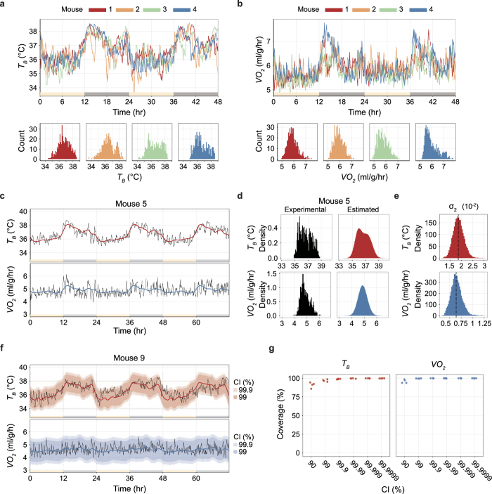
Figure 2. Modelling and predicting metabolism from a single day recording.

(a,b) The distribution of the T_B (a) and VO₂ (b) of four animals (mice 1 to 4) kept at a T_A of 12 °C for two days. The upper panels show the time series; light and dark periods are indicated by yellow and grey bars along the horizontal axis. The distribution for each animal is shown in the lower panels; each colour represents a different animal. (c) The estimated baseline metabolism dynamics of mouse 5. The mouse was kept at a T_A of 16 °C for three days. The baseline dynamics for 24 hours were fitted from the three-day-length data, and the standard deviation of the error (σ₂) for both T_B and VO₂ was estimated. The red and blue lines denote the median of the posterior distribution of the estimated T_B and VO_2, respectively. The data for the remaining three animals (mice 6 to 8) are available in Supplementary Fig. 2a. (d) The probability density of the experimentally obtained and estimated data for T_B and VO₂ for mouse 5. Black histograms represent experimental data; red and blue histograms show the estimated probability density. The data for mice 6 to 8 are available in Supplementary Fig. 2b. (e) The distribution of the estimated σ₂, which is the standard deviation of the error of the secondary trend, for T_B and VO₂. (f) The estimated baseline metabolism dynamics of mouse 9 with credible intervals (CIs). The T_A was kept at 16 °C for three days. The first 24 hours were used for estimation. The red and blue lines denote the median of the posterior distribution of the estimated T_B and VO₂. The red and blue shaded areas denote the CI. The data for mice 10 to12 are available in Supplementary Fig. 2c. (g) CI coverage rate of the metabolism on the second and third days when applying different CI ratios. The estimation was based on the first day. For both T_B and VO₂, 99.9% of the CIs covered more than 99% of the sampling points of the latter two days.