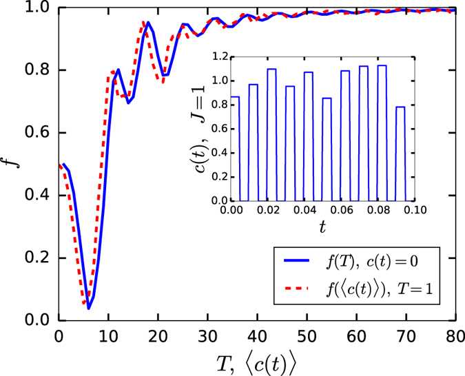
Figure 1. Quality factor f as a function of the time T as shown by the blue curve, where T > 60 roughly corresponds to the conventional adiabatic condition for our model, and as a function of the average control strength 〈c(t)〉 for T = 1 in the nonadibabtic domain.

The control c(t) is modelled as a train of pseudo-periodical square pulses with a fixed period 2Δt and duty cycle 50% (see example of c(t) in inset). The amplitude of the control pulses is given by J(1 − p(1/2 − r)), where r ∈ [0, 1) is a uniform random number, J > 0 is a parameter, and p describes the randomness of the control (we use p = 0.5 and Δt = 0.005). The Berry phase is numerically calculated by . Here we used a = 0.7605 and γ₁ = π/2.