Volumetry of low-contrast liver lesions with CT: Investigation of estimation uncertainties in a phantom study

Abstract

Purpose:

To evaluate the performance of lesion volumetry in hepatic CT as a function of various imaging acquisition parameters.

Methods:

An anthropomorphic abdominal phantom with removable liver inserts was designed for this study. Two liver inserts, each containing 19 synthetic lesions with varying diameter (6–40 mm), shape, contrast (10–65 HU), and both homogenous and mixed-density were designed to have background and lesion CT values corresponding to arterial and portal-venous phase imaging, respectively. The two phantoms were scanned using two commercial CT scanners (GE 750 HD and Siemens Biograph mCT) across a set of imaging protocols (four slice thicknesses, three effective mAs, two convolution kernels, two pitches). Two repeated scans were collected for each imaging protocol. All scans were analyzed using a matched-filter estimator for volume estimation, resulting in 6080 volume measurements across all of the synthetic lesions in the two liver phantoms. A subset of portal venous phase scans was also analyzed using a semi-automatic segmentation algorithm, resulting in about 900 additional volume measurements. Lesions associated with large measurement error (quantified by root mean square error) for most imaging protocols were considered not measurable by the volume estimation tools and excluded for the statistical analyses. Imaging protocols were grouped into distinct imaging conditions based on ANOVA analysis of factors for repeatability testing. Statistical analyses, including overall linearity analysis, grouped bias analysis with standard deviation evaluation, and repeatability analysis, were performed to assess the accuracy and precision of the liver lesion volume biomarker.

Results:

Lesions with lower contrast and size ≤10 mm were associated with higher measurement error and were excluded from further analysis. Lesion size, contrast, imaging slice thickness, dose, and scanner were found to be factors substantially influencing volume estimation. Twenty-four distinct repeatable imaging conditions were determined as protocols for each scanner with a fixed slice thickness and dose. For the matched-filter estimation approach, strong linearity was observed for all imaging data for lesions ≥20 mm. For the Siemens scanner with 50 mAs effective dose at 0.6 mm slice thickness, grouped bias was about −10%. For all other repeatable imaging conditions with both scanners, grouped biases were low (−3%–3%). There was a trend of increasing standard deviation with decreasing dose. For each fixed dose, the standard deviations were similar among the three larger slice thicknesses (1.25, 2.5, 5 mm for GE, 1.5, 3, 5 mm for Siemens). Repeatability coefficients ranged from about 8% to 75% and showed similar trend to grouped standard deviation. For the segmentation approach, the results led to similar conclusions for both lesion characteristic factors and imaging factors but with increasing magnitude in all the error metrics assessed.

Conclusions:

Results showed that liver lesion volumetry was strongly dependent on lesion size, contrast, acquisition dose, and their interactions. The overall performances were similar for images reconstructed with larger slice thicknesses, clinically used pitches, kernels, and doses. Conditions that yielded repeatable measurements were identified and they agreed with the Quantitative Imaging Biomarker Alliance’s (QIBA) profile requirements in general. The authors’ findings also suggest potential refinements to these guidelines for the tumor volume biomarker, especially for soft-tissue lesions.

1. INTRODUCTION

Quantitative imaging biomarkers (QIB) correlate with clinical outcomes and can be used to improve patient care.¹ More focus has been placed on standardization and validation of QIB through the collaboration of research, industry, and clinical practice in groups such as the Quantitative Imaging Biomarker Alliance (QIBA) of the Radiological Society of North America and the Quantitative Imaging Network (QIN) of the National Cancer Institute. These organizations seek to streamline the incorporation and evaluation of QIB in clinical trials, ultimately improving personalized precision medicine.

The size of a lesion is a useful biomarker for performing diagnosis, determining tumor progression, and monitoring response to treatment.^2–4 The most commonly used standard for characterization of lesion size is the Response Evaluation Criteria In Solid Tumors (RECIST), which requires a 1D measurement (diameter) of the tumor.⁵ In 2002, an initial study found that evaluating treatment response by volumetric measurement of liver lesions led to different results than evaluating response using 1D or 2D measurement.⁶ Later, an update to RECIST called for more validation, standardization, and wide-spread availability of volumetric methods before the adoption of these methods for routine use. Since then, there have been studies of lesions in phantoms, in the lung, and in the gastrointestinal tract that have demonstrated that volume better discriminates changes in lesion size.^7–10 For the liver, a 2012 study by Chalian et al. concluded that measurement of volumetric attenuation was reproducible in a study of 208 patients, and that it might be a better method of assessing changes of tumors in response to therapy.¹¹ However, factors contributing to variability in measuring the volume remained to be tested.

The uncertainties of the volume measurement process must be understood before QIB can be fully utilized. Estimation error depends on a number of factors including acquisition and reconstruction parameters, lesion characteristics, and estimation methods.^12–14 Imaging of in vivo lesions can only be performed for a limited range of acquisition factors due to CT radiation dose concerns for the patients. Zhao et al. studied the effects of slice thickness and reconstruction algorithm on tumor measurements from repeat CT scans, including the volume for lung, liver, and lymph node diseases in patients.^15,16 The use of phantoms allows for a wider range of factors to be systematically explored. Li et al. investigated many of these factors (lesion size, shape; scan exposure, slice thickness) using an anthropomorphic lung phantom and applied statistical analyses to the volume of the nodules.¹⁷ However, the estimation of liver lesion volume differs from the estimation of lung nodule volume due to much lower lesion-to-background contrast and higher noise levels. Furthermore, liver lesion contrast varies depending on the timing of the image acquisition with respect to the intravenous contrast agent injection (arterial phase ∼35 s after injection, portal-venous phase ∼75 s after injection). Investigation of volumetric estimation uncertainties for liver lesions may provide new insight into the design of studies examining volumetry of other types of soft tissue lesions and soft tissue lesions in general.

In this work, we investigated the influence of numerous factors in CT volumetry of liver lesions through a well-controlled phantom study. We applied statistical analyses to over 6000 measurements of lesion volume to determine the interaction of various imaging factors and the reliability of the QIB estimation. The phantom design, imaging protocol, volume estimators, and statistical methods are described in Sec. 2. In Sec. 3, the results are presented, followed by a discussion in Sec. 4, and conclusion in Sec. 5.

2. MATERIALS AND METHODS

2.A. Phantom design

An anthropomorphic abdominal phantom with a removable liver insert was designed by the research team and custom manufactured by QRM (Moehrendorf, Germany). Two inserts containing 19 lesions each were made to simulate arterial and portal-venous phase imaging of the liver. For the arterial phase, the liver parenchyma was nominally uniform at 80 HU, with CT values ranging between 60 and 120 HU for the various synthetic liver lesions. For the portal-venous phase, the CT value for the liver parenchyma was 110 HU, and the lesion CT values ranged between 45 and 100 HU. Table I contains a list of the synthetic lesion properties of the inserts. Eight lesion sizes (6, 8, 10, 20, 23, 30, 34, 40 mm diameter) and three shapes (spherical, ellipsoidal, and lobulated), both solid and mixed density, were included in the liver inserts. The lesion-to-background contrast (absolute value of HU difference between lesion and surrounding parenchyma) ranged from 10 to 40 HU for the arterial phase and 10–65 HU for the portal-venous phase, where contrast is defined as the absolute difference between the background and the lesion. A previous study has shown that a minimum of 10 HU is required to observe the lesion.¹⁸ Figure 1 shows the schematic of the phantom. The reference standard volume for the lesion was provided by QRM and was measured prior to final insertion with the liver inserts.

TABLE I.

A table of lesion characteristics including nominal lesion density and contrast values for the arterial and portal venous phase liver inserts at 120 kVp. The nominal radiodensity of liver parenchyma is 80 HU for the arterial phase and 110 HU for the portal venous phase insert at 120 kVp. Lesions 5–6 and 11–12 refer to mixed density objects with specified outer/inner properties.

Lesion index				Lesion density (HU)		Contrast (HU)
Arterial	Venous	Diameter (mm)	Shape	Arterial	Venous	Arterial	Venous
1	20	34	Lobulated	60	45	20	65
2	21	34	Lobulated	120	75	40	35
3	22	30	Ellipsoid	60	45	20	65
4	23	30	Ellipsoid	120	75	40	35
5	24	30/20	Spherical/spherical	100/45	90/45	20	20
6	25	30/20	Spherical/spherical	90/120	100/60	10	10
7	26	23	Lobulated	60	45	20	65
8	27	23	Lobulated	120	75	40	35
9	28	20	Ellipsoid	60	45	20	65
10	29	20	Ellipsoid	120	75	40	35
11	30	20/10	Spherical/spherical	100/45	90/45	20	20
12	31	20/10	Spherical/spherical	90/120	100/60	10	10
13	32	40	Ellipsoid	90	100	10	10
14	33	10	Spherical	60	75	20	35
15	34	10	Spherical	90	90	10	20
16	35	8	Spherical	60	75	20	35
17	36	8	Spherical	90	90	10	20
18	37	6	Spherical	60	75	20	35
19	38	6	Spherical	90	90	10	20

FIG. 1.

Layout of the anthropomorphic abdominal phantom and liver inserts with fixed built-in lesions. The arterial and portal venous phase liver inserts had the same lesion layout.

2.B. Imaging protocols

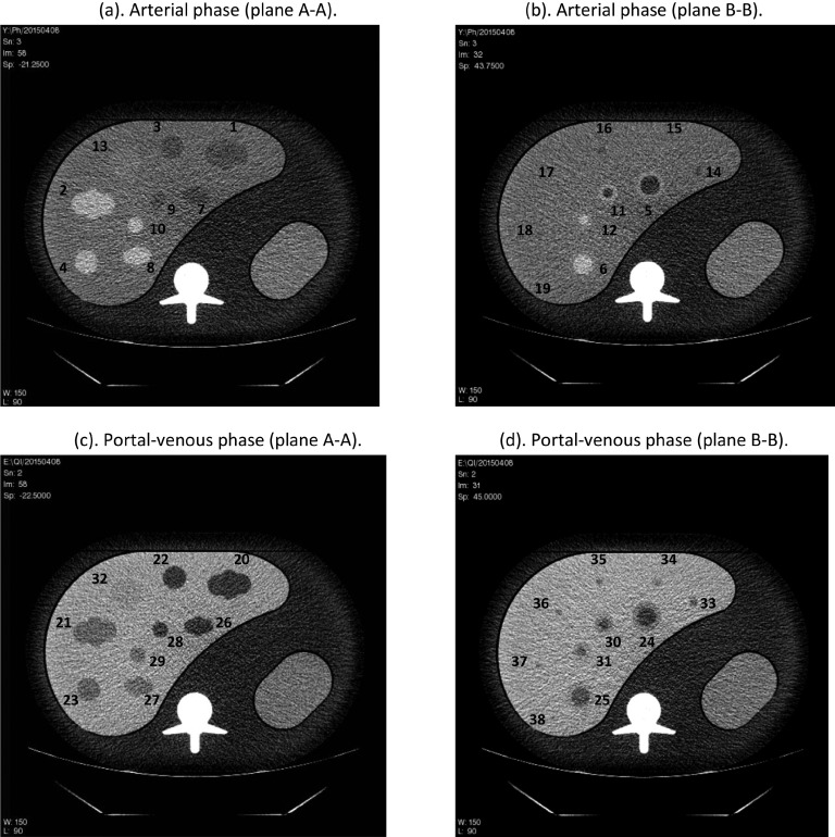
Imaging protocols utilized in this study are given in Table II. The phantom was imaged at the Columbia University Medical Center with two 64-slice multi-detector helical CT scanners: GE 750HD (GE Healthcare, Chicago, IL, US) and Siemens Biograph mCT (Siemens Healthcare, Erlangen, Germany). The data were acquired at 120 kVp and at three dose levels of approximately 3.8, 7.6, and 19 mGy corresponding to 50, 100, and 250 effective tube current time product (mAs), respectively. Effective mAs is defined as (total mAs)/pitch for the scan. There are small differences between the acquired pitch and associated slice thicknesses between the two CT systems as the available setting of these two imaging parameters is different for these two CT scanners. For the GE system, we acquired pitch factors of 1.375 and 0.983; for the Siemens system we acquired pitch factors of 1.35 and 1.0. The mAs was adjusted for each pitch to reach the three pre-set effective mAs. CT acquisitions for the Siemens image data acquired at a pitch of 1.0 were collected for only a single dose of 250 effective mAs. The GE image data were reconstructed at slice thicknesses of 5.0, 2.5, 1.25, and 0.625 mm and the Siemens data were reconstructed at 5.0, 3.0, 1.5, and 0.6 mm. Filtered back-projection (FBP) reconstructions were used with two different kernels from each vendor’s scanner: GE, Standard and Soft and for Siemens, correspondingly, B30f and B20f. For each liver insert (arterial, portal-venous), data from two repeated scans were collected. Figure 2 shows four example images corresponding to plane A-A and B-B from Fig. 1 for both the arterial and the portal venous phase with lesion indexes labeled.

TABLE II.

CT imaging protocols for the anthropomorphic liver phantom. Two repeated scans were acquired for each imaging acquisition condition.

	Acquisition parameters				Reconstruction parameters
Scanner	kVp	Eff. mAs	Pitch	Collimation	Slice thickness	Overlap	Recon algorithm	Convolution kernel
GE 750HD	120	50	1.375	64 × 0.625	5	0%	FBP	Standard
		100	0.983		2.5			Soft
		250			1.25
					0.625
Siemens mCT	120	50	1.35	64 × 0.6	5	0%	FBP	B30f
		100	1.0a	(32 × 0.6 detector width)	3.0			B20f
		250			1.5
					0.6

^aOnly one effective mAs (250) was acquired for pitch 1.0.

FIG. 2.

Example CT slices of the abdominal phantom containing either the arterial [(a) and (b)] or portal venous [(c) and (d)] phase liver insert (250 effective mAs, slice thickness 2.5 mm, GE 750HD). Note that some small lesions in (b) are not visible at this window level.

In total, we collected 320 image series (i.e., GE: 48 imaging protocols ×2 repeats ×2 phantoms; Siemens: 32 imaging protocols ×2 repeats ×2 phantoms) and 34.4 GB image data. All of the acquired image data are ready to be submitted to the quantitative imaging data warehouse (QIDW), the RSNA/QIBA designated data warehouse.

2.C. Volume estimation

Two noncommercial volume estimation tools were used. The first was a model-based matched-filter (MF) volume estimator.¹⁹ It is unsupervised (i.e., no human corrections were applied) and assumes prior knowledge of the general location (a seed point) and the shape for each lesion. For mixed density lesions, volume measurements were made for the entire object. More details on the matched-filter method can be found in the Appendix. The second algorithm is based on a marker-controlled watershed segmentation (SEG) approach developed for segmentation of hypo-intense liver lesions.¹³ It required manual selection of a region-of-interest inside the lesion on one image to initiate the segmentation. The algorithm then automatically found lesion boundaries on all image series containing the 3D lesion. For the segmentation approach, a radiologist also reviewed every segmentation and made modifications using a noncommercial editing tool when necessary.

The matched-filter estimator was applied to all 320 image series, resulting in 6080 volume measurements (320 × 38 lesions). The segmentation estimator was applied on a subset of data: portal-venous insert lesions, 250 mAs with GE and 250 mAs with Siemens at pitch 1.0, resulting in 912 measurements.

2.D. Statistical analysis methods

2.D.1. Analyses on matched-filter results

Prior to analyses, all data were log-transformed (natural log) to reduce the heteroscedastic nature that was observed in our volumetric measurements (variance of the measurements increased substantially with larger lesions without this transformation). We applied N-way ANOVA with two-way interaction for factor analysis on all measurements, using lesion size, lesion contrast, effective mAs (dose), slice thickness, convolution kernel, and scanner as factors. We used type II sums of squares for ANOVA analysis. Lesion shape was not included since it was highly correlated with lesion size (small lesions are all spherical, see Table I). For slice thickness, 0.6 and 0.625 mm, 1.25 and 1.5 mm, and 2.5 and 3 mm were treated as the same category, respectively. For a convolution kernel, standard and B30f and soft and B20f were treaded as the same category, respectively. Based on the ANOVA results, statistically significant imaging parameters were considered major parameters. The others were referred to as minor parameters. Measurements were then pooled for root mean square error (RMSE) evaluation if they were from imaging protocols with the same major parameters, where the error was defined as the volume error (difference between the volume measurement and the reference standard). Lesions that were associated with high RMSE were visually inspected to determine if they were not measurable or likely to be disqualified in practice for the estimation task. Those lesions were then excluded for the rest of the analyses.

Same ANOVA analysis was applied again on the measurements of the remaining data. Since two ANOVA analyses were applied on an overlapping dataset, p-value was set to 0.025 according to Bonferroni correction. Significant factors were identified and ranked according to eta-squared, which was calculated as the ratio of the between-group sum of squares to the total sum of squares.¹⁷ Distinct repeatable imaging conditions were also determined based on the ANOVA results. Imaging protocols that only differed in minor parameters were grouped to define a repeatable imaging condition.

Statistical analyses were done based on the metrology recommendations outlined by the QIBA metrology working group, which included the analysis of linearity, bias with standard deviation, and repeatability.^20–22 Overall linearity was assessed by linear regression. Regression slope and intercept with 95% confidence interval (CI) were reported. Grouped bias with standard deviation was reported for each repeatable imaging condition. Repeatability was evaluated as repeatability coefficient for each repeatable imaging condition, with lower value indicating better repeatability.

For a repeatable imaging condition, let y_ijk be the volume measurement for each lesion i = 1, 2, …n, each combination of minor parameters within the repeatable imaging condition j = 1, 2, …m, and each repeated measurement k = 1, 2. Let x_i be the reference standard volume. The mean measurement for the ith lesion in log domain is then

$${\displaystyle {\mu }_i=\frac{1}{2m}\sum _{j,k}ln{y}_{ijk}}$$

and the error compared to the reference standard is

$${\displaystyle e_{ijk}=ln{y}_{ijk}-ln{x}_i.}$$

Grouped bias for the repeatable imaging condition was calculated as

$${\displaystyle B=\frac{1}{2nm}\sum _{i,j,k}{e}_{ijk},}$$

and standard deviation as

$${\displaystyle {\sigma }_e=\sqrt{\frac{1}{2nm-1}\sum _{i,k,j}{\left(e_{ijk}-B\right)}^2}.}$$

The repeatability coefficient (RC) was defined as 2.77 σ_w, where the within-subject variance ${\sigma }_w^2$ was calculated as the mean over all lesions of the variance over all combinations of minor parameters and repeated measurements,

$${\displaystyle {\sigma }_w^2=\frac{1}{n}\sum _i\left(\frac{1}{2m-1}\sum _{k,j}{\left(ln{y}_{ijk}-{\mu }_i\right)}^2\right).}$$

All the results in log units were converted to and reported in percentage in the base unit of measurement.¹⁷ More details for each performance metric used as part of this analysis can be found in previous work.^17,20

2.D.2. Analysis on segmentation results

The same metrics described above for the matched-filter results were also used to evaluate the segmentation results.

3. RESULTS

3.A. MF results

3.A.1. Determine lesions to exclude and imaging protocols to pool

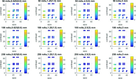
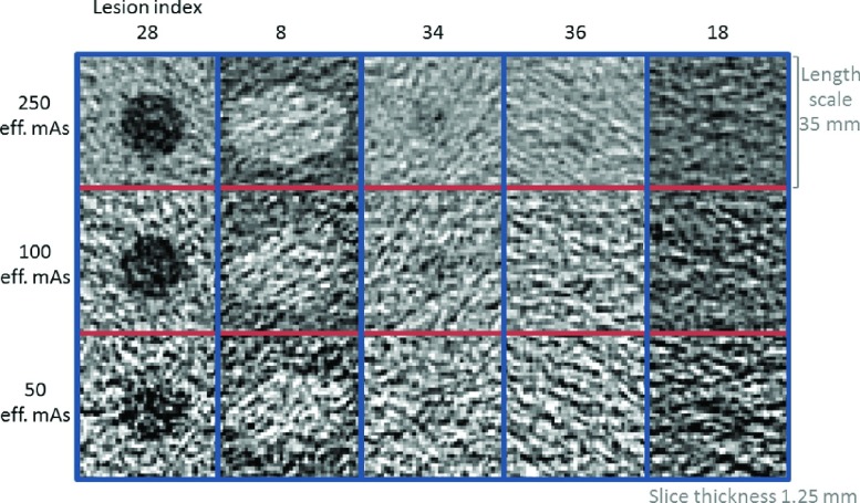
Applying N-way ANOVA with two-way interaction (six factors: dose, kernel, slice thickness, scanner, size, and contrast) to all MF volume measurements, we identified the following statistically significant factors: size, size × slice thickness, size × dose, size × contrast, dose, slice thickness, (p < 0.025, interacting factors indicated by ×). Based on those results, further analysis was conducted across dose and slice thickness, whereas kernel and scanner were pooled together. For each of those imaging conditions, RMSEs were evaluated for each of the 38 lesions. Figure 3 summarizes the RMSE results. Clearly, the lesions ≤10 mm (lesions 14–19, 33–38) were associated with large errors for most of the imaging protocols. For these lesions, there were 1920 measurements, and among those, 338 measurements were on the limits of the MF search range (see the Appendix). Therefore, we considered these lesions as not reliably measurable for our MF algorithm. Visual inspection of the images also confirmed the difficulty in detecting these lesions or identifying the boundary of the lesions (Fig. 4). These small (≤10 mm) lesions were all excluded, although the 10 mm lesion with +35 HU contrast (index 33) yielded low RMSE for one or two imaging conditions with 250 effective mAs. For the rest of the large lesions (≥20 mm), only 30 out of 4160 were on the limits of the MF search range, which were mostly associated with the lowest dose and the thinnest slice thickness protocols and involved small or low contrast lesions. For the purpose of keeping data more balanced, those cases were not excluded.

FIG. 3.

RMSEs for all lesions across mAs (each row) and slice thickness (each column). Each dot represents the lesion with corresponding size and contrast (overlapped dots are slightly shifted) with color reflecting the RMSE magnitude. Lesions ≤10 mm are shown within the dotted-box in the first plot.

FIG. 4.

Center slice images from example lesions. Lesions 34, 36, and 18 were ≤10 mm and were excluded as described in Sec. 3.A.1. Lesions 28 and 8 were ≥20 mm and were included, but degraded image quality is noticeable over reduced dose. The example images are from a GE dataset with 1.25 mm slice thickness and standard reconstruction kernel.

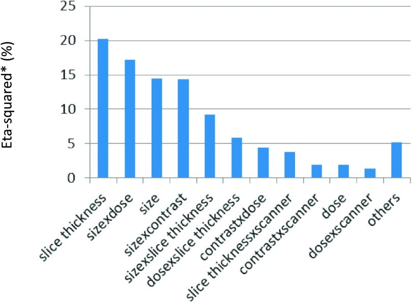
Applying the same ANOVA analysis on large lesions, slice thickness, size × dose, size, size × contrast, size × slice thickness, dose × slice thickness, contrast × dose, slice thickness × scanner, contrast × scanner, dose, and dose × scanner were found statistically significant. Eta-squared was calculated for each factor and scaled so that summation of the adjusted eta-squared was 100%. The adjusted eta-squared for all the significant factors and the others combined is shown in Fig. 5. Slice thickness turned out to be the most dominant factor since some low contrast lesions had large errors with thin slice thickness. Finally, 24 distinct imaging conditions were defined for repeatability testing based imaging protocols with the same slice thickness, dose, and scanner (4 slice thicknesses × 3 doses × 2 scanners).

FIG. 5.

Adjusted eta-squared in percentage for all significant factors and the others combined for the MF volume estimator.

3.A.2. Linearity

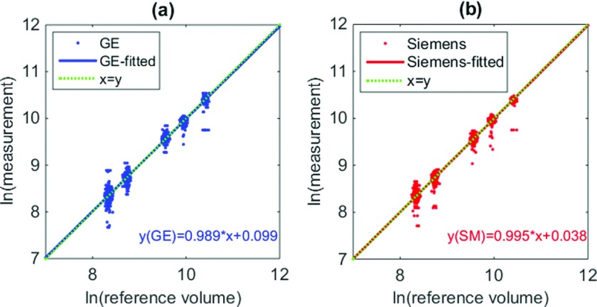
Scatter plot of the data (measurements versus reference standard) and the linear regression lines is given in Fig. 6. Note that separate analyses were conducted for each scanner since the interaction between scanner and slice thickness, contrast, and dose was found to be of significant factors by ANOVA. For GE, the slope and intercept of the regression line were 0.989 (95% CI [0.984, 0.994]) and 0.099 (95% CI [0.055 0.144]), respectively. For Siemens, the slope and intercept of the regression line were 0.995 (95% CI [0.989, 1.002]) and 0.038 (95% CI [−0.020 0.097]), respectively. For both scanners, the regression lines were close to the diagonal, indicating good linear relationship between measurements and reference standard, and on average results in low biased estimates.

FIG. 6.

Scatter plot for the reference standard and measurements (in log domain) for (a) GE and (b) Siemens scanner. Blue/red lines in plot (a)/(b) correspond to the regression lines for GE and Siemens data, respectively, which aligned well with the diagonal (green-dotted) line. Note that a small random offset was added to the x-coordinate of each point (reference standard) to avoid over-plotting of the data points.

3.A.3. Grouped bias analysis

Table III summarized biases and standard deviations for all large lesions with each repeatable imaging condition. We observed overall low biases (within −3.04% to 2.30%) except for the Siemens, 0.6 mm, 50 eff. mAs imaging condition, for which bias was about −10%. There was a trend of increasing standard deviation with decreasing dose. For each fixed dose, the standard deviations were similar among the three larger slice thicknesses (1.25, 2.5, 5 mm for GE, 1.5, 3, 5 mm for Siemens). Standard deviations were highest for the smallest slice thickness and decreasing dose, indicating a possible benefit of larger slice thickness for this low-contrast task to reduce noise through data averaging.

TABLE III.

Biases ± standard deviations (in %) for measurements imaged with the three doses coupled with the four slice thicknesses for each scanner.

	GE				Siemens
	0.625 (mm)	1.25 (mm)	2.5 (mm)	5 (mm)	0.6 (mm)	1.5 (mm)	3 (mm)	5 (mm)
250 eff. mAs	−0.42	−0.53	0.50	0.88	−1.16	−0.11	0.51	1.39
	±4.57	±4.42	±4.27	±6.08	±8.22	±3.74	±3.73	±4.03
100 eff. mAs	−2.39	−0.67	0.51	2.13	−3.04	0.13	1.07	1.81
	±11.80	±5.85	±5.42	±6.82	±14.82	±6.77	6.09	±6.53
50 eff. mAs	−2.09	−1.84	0.39	2.30	−9.67	−0.34	0.47	1.47
	±16.56	±13.55	±9.96	±9.80	±25.91	±7.28	±9.21	±10.74

3.A.4. Repeatability

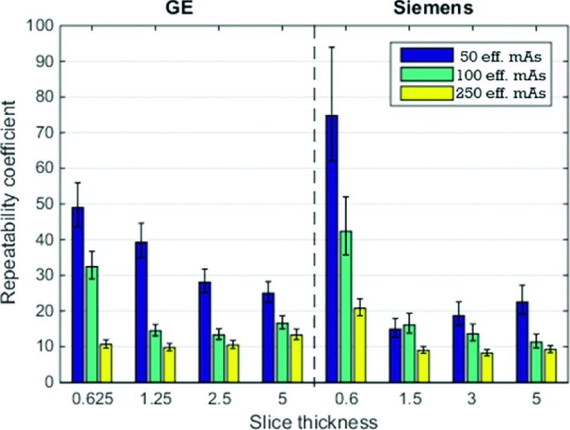
Similar to bias and variance analysis, we evaluated the repeatability coefficients for each repeatable imaging condition. Results are shown in Fig. 7. The performances between the two scanners were comparable for imaging conditions associated with lower noise (higher mAs and larger slice thicknesses). Slice thickness influenced the repeatability but there was no clear pattern. With 250 mAs, repeatability coefficients for all slice thicknesses were similar for GE and repeatability coefficients for slice thicknesses larger or equal to 1.5 mm were similar for Siemens. As far as dose was concerned, there was a general decreasing trend in the repeatability coefficient (i.e., better repeatability) with increasing dose.

FIG. 7.

Plots of repeatability coefficients (in %). The 95% CI are indicated by error bars.

3.B. SEG results

In this section, measurements obtained by the semi-automatic segmentation algorithm are analyzed.

The segmentation algorithm (without human correction) failed to segment most small lesions (≤10 mm). When that happened, the radiologist manually segmented the lesion. The segmentation also failed for a number of thin slice thickness scans and among those, there were two cases where the radiologist (M.Z.) could not detect any lesion. The radiologist also reported that when he measured the lesions from images acquired on the Siemens scanner at first, he had little or no knowledge about the lesion characteristics, whereas he was much more aware of the lesion characteristics when segmenting the lesion from the GE images at a later time. In particular, for the mixed-density lesions (lesion 24, 25, 30, 31), he was more certain that those lesions had a low contrast ring outside of the inner sphere. Therefore, we observed very inconsistent measurements for those lesions across the two scanners. Especially for lesion 25 and 31, where the outer shell of the lesions had a contrast of 10 HU, the radiologist’s performance was substantially improved for the GE scan data segmented at a later time. As such, the mixed-density lesions were excluded from analysis.

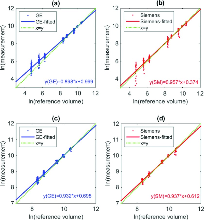
Linearity of segmentation results is shown in Fig. 8. In Figs. 8(a) and 8(b), all measurements for homogenous lesions were included. Again, small lesions were associated with large errors. Figures 8(c) and 8(d) show the results with large homogenous lesions only. The slopes were significantly different from 1 and the intercepts significantly different from 0 (p < 0.05) for the segmentation-based estimates.

FIG. 8.

Scatter plot for the reference standard and measurements (in log domain) for [(a) and (b)] all segmentation results [(c) and (d)] homogenous large lesions for GE and Siemens, respectively. Dotted and solid lines correspond to the diagonal line, regression lines for GE or Siemens data, respectively.

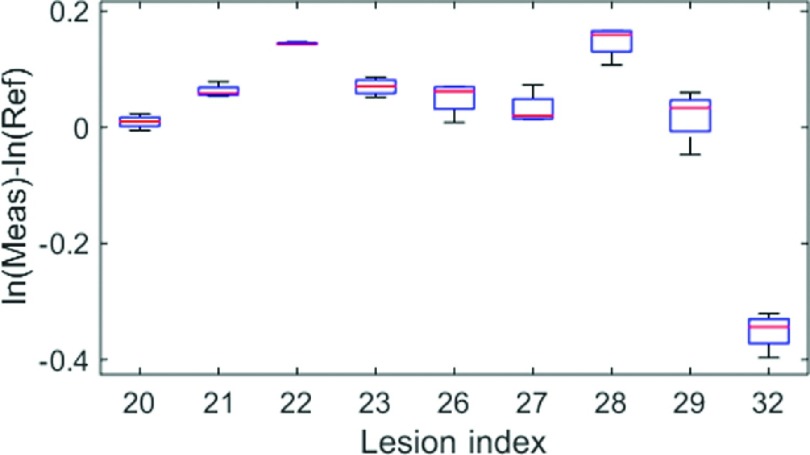
For homogenous large lesions, we ended up with 430 measurements. We evaluated the grouped biases and standard deviations, and the repeatability coefficients for each scanner with each slice thickness. The results are reported in Tables IV and V. For bias and standard deviation, the middle range slice thicknesses (1.25, 1.5, 2.5, 3 mm) yielded relatively better results than the others. Unlike for the matched-filter approach, the pattern for repeatability coefficients with different slice thicknesses was different from what was observed for the grouped standard deviation. For instance, for Siemens with a 0.6 mm slice thickness reconstruction, the standard deviation was the highest among all slice thicknesses, but it also yielded the best repeatability. A close inspection of the measurements for each lesion (Fig. 9) showed that there was large between-subject variability (i.e., biases for some lesions were substantially different than others). Thus, the grouped standard deviation was large. However, within-subject variability was small so that the measurements were quite repeatable. Recall that according to linearity analysis, the slope was not particularly close to 1 so it was not surprising to see large between-subject variability.

TABLE IV.

Biases ± standard deviations (in %) for measurements of large homogenous lesions across the four slice thicknesses for each scanner.

Scanner	GE				Siemens
Slice thickness (mm)	0.625	1.25	2.5	5	0.6	1.5	3	5
Biases	12.49	4.88	1.61	9.86	2.08	−2.71	−0.43	11.34
±stdev	±12.01	±6.29	±7.85	±9.97	±15.40	±7.80	±8.05	±6.34

TABLE V.

Repeatability coefficients (in %) for measurements of large homogenous lesions across the four slice thicknesses for each scanner: (a) GE, (b) Siemens.

(a)
Scanner	GE
Slice thickness (mm)	0.625	1.25	2.5	5
Repeatability coefficient (%)	12.25	7.58	20.74	20.83
95% CI	[10.35,15.03]	[6.42,17.42]	[17.42,25.65]	[17.49,25.75]
(b)
Scanner	Siemens
Slice thickness (mm)	0.6	1.5	3	5
Repeatability coefficient (%)	7.47	11.00	13.13	9.16
95% CI	[5.86,10.30]	[8.60,15.27]	[10.25,18.29]	[7.17,12.66]

FIG. 9.

Boxplot for differences between measurement and reference standard (in log) for each lesion. Data are from Siemens scans with 0.6 mm slice reconstruction and 250 effective mAs.

4. DISCUSSION

In this study, we examined the volumetry of liver lesions with CT, using images of an anthropomorphic liver phantom acquired with various imaging protocols. Volume measurements for lesions of multiple sizes and contrasts were extracted using two estimation tools. The two estimation tools were selected such that the matched-filter method could serve as a performance bound whereas the semi-automatic approach with a radiologist correction would better represent expected results in clinical practice. In this section, we will discuss the main findings of this study and their connection to QIBA’s current CT Tumor Volume Change Profile on measuring tumor volume and volume change.²³

For both estimation approaches, we found that the performance of lesion volume estimation was strongly dependent on lesion size, lesion-to-background contrast, acquisition dose, and their interactions. Due to the high noise levels associated with abdominal scans, liver lesions that were less or equal to 10 mm in diameter were found to be too difficult to estimate, even at clinically realistic dose levels. For lesions of size 20 mm or larger, the performance depended on the lesion contrast, size, and CT dose. Higher contrast, larger size, and higher dose yielded more accurate and precise measurements. The semi-automated segmentation approach also failed often for small lesions and thin slice scans. The radiologist reported that the scans from lower doses were too noisy to work with, meaning that only the 250 effective mAs dataset was measured for the semi-automated approach. As such, lower dose degraded the estimation performance for segmentation approach too.

The main claim of QIBA’s CT Tumor Volume Change Profile states that “a measured increase in mass volume of 30% or more indicates that a true increase has occurred with 95% confidence,” which was based on the clinical performance target. For that performance target to be achieved, the tumor is required to be measurable and the longest in-plane diameter is between 10 and 100 mm. The lesion contrast has not been explicitly addressed in the profile, but lesions with very low contrast probably would fail the qualitative “measurability” criteria in the QIBA Profile so the Profile would likely not be applicable to these lesions. Our results suggested that it is likely important to consider at least the lesion’s size and contrast in determining which lesions are appropriately measurable within the QIBA Profile. Lesion contrast was found to be much less important for lung nodules because the contrast between a lung nodule and the background lung parenchyma is typically much larger than that found between a liver lesion and the liver background. The importance of both size and contrast could potentially be used to make the QIBA definition of “measurable” more systematic to apply.

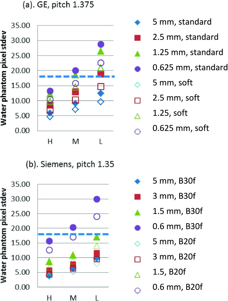
In addition to lesion characteristics, imaging parameters more or less influence the image quality and impact the performance of the volume estimation. However, the “best” imaging conditions are task-based and are not easy to standardize, since changes in each parameter to gain certain benefits often lead to some sacrifice in other aspects. For instance, increasing dose reduces image noise but poses additional patient risks, increasing slice thickness reduces image noise but leads to lower spatial resolution along the z-axis, changes in reconstruction kernel are associated with trade-off between image noise and spatial resolution, to name a few. To achieve the clinical performance target in QIBA’s claim, the Profile also has requirements on the imaging protocols in addition to lesion characteristics. They included but are not limit to the following: (1) the standard deviation for the central region of a uniform 20 cm cylindrical water phantom should be no greater than 18 HU; (2) the reconstruction kernel shall be consistent (for scans of different time points to measure change); and (3) slice thickness shall be set to less than or equal to 1.5 mm. We evaluated the pixel standard deviation and the results are shown in Fig. 10. We found that, in general, the imaging conditions resulting in poor repeatability (large repeatability coefficient) (Fig. 7) corresponded to those with pixel noise higher than 18 HU. Regarding the reconstruction kernel, no impact on measurements was found for either volume estimation method, although different kernels led to quite different noise levels. In comparison to the standard/B30f kernel (GE/Siemens), the small noise reduction provided by the soft/B20f kernel (GE/Siemens) is accompanied by a small sacrifice in spatial resolution. These two competing effects appear to basically offset each other resulting in no appreciable change in the overall performance of the volume estimation. In this work, we chose the standard (B30f) and soft (B20f) kernels as they are commonly used in clinical practice for abdominal studies. Our results suggested that the standard (B30f) and soft (B20f) kernel could be used interchangeably. Finally, for slice thickness, our data suggest a less restrictive requirement than that of the QIBA’s Profile, which could be appropriate when sizing liver lesions. In particular, at 250 effective mAs, slice thicknesses of 0.625, 1.25, and 2.5 mm for GE and slice thicknesses of 1.5, 3, and 5 mm for Siemens yielded similar performances in terms of overall bias, variance, and repeatability for the matched-filter estimation approach. For segmentation results, slice thickness of 2.5 mm for GE and 3 mm for Siemens also yielded similar or better performance compared to those from smaller slice thicknesses scans. With 5 mm slice thickness, the repeatability coefficients for both scanners were below 30%, which is the clinical target of QIBA’s CT Tumor Volume Change Profile. One reason that large slice thicknesses produced relatively small error in this study is that the lesions qualified for measuring were 20 mm or larger, which is typical for liver lesions in clinical practice. In addition, images with larger slice thickness produced less noisy scans, which was found to be especially important for low-contrast lesions in the liver. In current clinical practice, protocols for abdominal CT scanning are typically thicker than 1.5 mm due to the high noise presented and the clinical interest in relatively large lesions in the liver. While this might change in the future with better imaging techniques, at the current stage, to perform lesion volume estimation in the abdomen area with reasonable dose, the QIBA’s CT Tumor Volume Change Profile might need to relax the requirement on the slice thickness.

FIG. 10.

Noise measurements of a water phantom for imaging protocols used in this study (pitch 1.0 for GE and 0.98 for Siemens were almost the same). H, M, and L on x-axis correspond to eff. mAs of 250, 100, and 50, respectively. The diameter of the water phantom is 21.6 cm and a region of interest of 400 mm² was used for standard deviation evaluation. The dashed line corresponds to 18 HU.

Finally, in this study, two estimation approaches were applied, one based on a matched-filter approach that was designed as a low-bias estimator and thus produced a bound on performance, and a segmentation-based method which better represented the performance expected in clinical practice. Results from matched-filter were indeed much better compared to segmentation results in terms of linearity, accuracy, and precision. For example, repeatability coefficients for the same dataset were smaller for matched-filter (Table VI versus Table V). The purpose here is not to compare the estimators but to investigate the source of variations and build a framework for protocol standardization and algorithm performance evaluation. More informed estimators such as the matched-filter method can be used to identify and test sources of variation from the imaging systems and measurement tools. Also, they could be used as part of an initial systematic test to determine if certain lesions are measurable since those deemed not measurable are expected to have a substantial degradation in volume estimation performance. Our segmentation results, on the other hand, may more closely approximate volume estimation tools currently available for use and also can incorporate an important additional source of variation coming from the clinician directly interacting with the segmentation tool.

TABLE VI.

Matched-filter results parallel to Table V: repeatability coefficients (in %) for measurements of large homogenous lesions imaged with the two scanners coupled with the four slice thicknesses.

Scanner	GE				Siemens
Slice thickness (mm)	0.625	1.25	2.5	5	0.6	1.5	3	5
Repeatability coefficient	7.68	5.50	4.82	5.73	4.99	4.84	6.27	5.31

There are limitations to our study. First, there was a size gap between 10 and 20 mm. We included lesions that were most clinically relevant in the liver (size 20 mm and larger) and the sub-centimeter lesions to investigate the limit of lesion size that could be reliably estimated. Our previous studies in the lung indicated that 10 mm lesions could be reliably estimated, unfortunately, it was not the case for low contrast liver lesions in this study. Supplemental studies with lesions within 10–20 mm size range should be performed. Second, while the x-ray spectrum is a key factor that impacts lesion contrast, which may lead to different estimation performance, kVp was fixed in our study. The 120 kVp setting was selected because it was thought to be most appropriate based on the physical size of the liver phantom and the fact that the reference lesion and parenchyma CT values given by the phantom manufacturer were based on 120 kVp. Clinically, different kVps are selected based on patient sizes. Since the effect of patient size is not within the scope of our study, we did not vary kVp. Adding fat rings to allow investigation of kVp is a potential addition to a future study. Third, FBP reconstruction was the only method evaluated in this study. As there is a strong need to investigate the impact iterative reconstruction algorithm’s on estimation, we are now conducting a study focusing on how iterative reconstruction impacts liver-lesion volume estimation. Fourth, only one radiologist did the manual correction to the semi-automatic segmentation. For that one reader, the reading order was not randomized. Thus the statistical power of the results for that approach was reduced. We plan to perform more analyses once we collect more segmentation results (better controlled readings, more radiologists).

5. CONCLUSION

In this work, we evaluate the performance of liver lesion volumetry in hepatic CT with various imaging parameters. Our results show that liver lesion volumetry is strongly dependent on lesion size and contrast, acquisition dose, and their interactions. The overall performances were similar for images reconstructed with larger slice thicknesses, clinically used pitches, kernels, and doses. Conditions that yielded repeatable measurements were identified and they agreed with the QIBA’s Profile requirement in general. Our findings also suggest potential refinements to these guidelines for the tumor volume biomarker, in particular the guidelines may be tailoring to different types of lesions, especially for soft-tissue lesions. However, any such tailored refinements need to be weighed against the simplicity of a single approach for all types of lesions.

APPENDIX: MATCHED-FILTER ESTIMATOR IMPLEMENTATION

The volumes of the lesions were estimated using a modification of the matched-filter-based method of Gavrielides et al.¹⁹ For each data acquisition, and for each target lesion, the method minimizes the difference between the lesion volume of interest and a collection of simulated 3D templates. These templates were generated by a model of the CT imaging system mapping from the object shape to the sinogram, and by filtered back-projection mapping from the sinogram to the image.²⁴ The templates vary in centroid-position, density, and size, as shown in Table VII.

TABLE VII.

Template variables for volume estimation. Initial estimates are determined prior to matching: centroid from manual estimation, background and lesion density from regions on the edge and center (respectively) of the volume of interest. The half-pixel offsets in x, y are created by repositioning the object prior to CT simulation, and the quarter-pixel offsets in z are created by decimating a high-resolution template.

Variable	Values	Step size
Centroid pixel offset	Initial estimate ± 3 pixels	0.5 pixels in x, y; 0.25 in z
Background density	Initial estimate ± 30 HU	1 HU
Lesion density	Initial estimate ± 20 HU	1 HU
Lesion size	80%–120% of ground truth diameter mm	1% of ground truth diameter mm

For each target lesion, there are over 5.6 × 10⁸ (13 x location × 13 y location × 25 z location × 61 background density × 41 lesion density × 41 diameter) possible configurations of the template (for mixed density lesions, there is an additional density and size variable leading to over 2.3 × 10¹⁰ configurations; note that sizes for both inner and entire objects are estimated but only the measurements for the entire objects are used in the analysis), and determining the optimal template from an exhaustive search is computationally prohibitive. Instead, we use a coordinate descent method known as Powell’s conjugate direction.²⁵ The objective function is minimized for each variable in sequence, followed by a minimization in the conjugate direction based on the net change. This process is iterated until convergence to a minimizing template. To account for noise in the image—which can lead to local minima—we begin the matched-filtering of each volume of interest with ten random initial conditions, run Powell’s method on each, and then choose the final template with the minimal cost function. Depending on the properties of the target data, we find that Powell’s method requires between 2 and 7 iterations to converge. In total, at most 9.8 × 10⁴ configurations are examined for each volume of interest using the iterative coordinate descent, several orders of magnitude lower than the exhaustive search.

CONFLICT OF INTEREST DISCLOSURE

The authors have no COI to report.

REFERENCES

- 1.Wang Y.-X. J. and Ng C. K., “The impact of quantitative imaging in medicine and surgery: Charting our course for the future,” Quant. Imaging Med. Surg. , 1–3 (2011). 10.3978/j.issn.2223-4292.2011.09.01 [DOI] [PMC free article] [PubMed] [Google Scholar]
- 2.Lencioni R. and Llovet J. M., “Modified RECIST (mRECIST) assessment for hepatocellular carcinoma,” Semin. Liver Dis. , 52–60 (2010). 10.1055/s-0030-1247132 [DOI] [PubMed] [Google Scholar]
- 3.Mitchell D. G., Bruix J., Sherman M., and Sirlin C. B., “LI-RADS (liver imaging reporting and data system): Summary, discussion, and consensus of the LI-RADS management working group and future directions,” Hepatology , 1056–1065 (2015). 10.1002/hep.27304 [DOI] [PubMed] [Google Scholar]
- 4.Gonzalez-Guindalini F. D., Botelho M. P. F., Harmath C. B., Sandrasegaran K., Miller F. H., Salem R., and Yaghmai V., “Assessment of liver tumor response to therapy: Role of quantitative imaging,” Radiographics , 1781–1800 (2013). 10.1148/rg.336135511 [DOI] [PubMed] [Google Scholar]
- 5.Therasse P., Arbuck S. G., Eisenhauer E. A., Wanders J., Kaplan R. S., Rubinstein L., Verweij J., Van Glabbeke M., van Oosterom A. T., Christian M. C., and Gwyther S. G., “New guidelines to evaluate the response to treatment in solid tumors. European Organization for Research and Treatment of Cancer, National Cancer Institute of the United States, National Cancer Institute of Canada,” J. Natl. Cancer Inst. , 205–216 (2000). 10.1093/jnci/92.3.205 [DOI] [PubMed] [Google Scholar]
- 6.Prasad S. R., Jhaveri K. S., Saini S., Hahn P. F., Halpern E. F., and Sumner J. E., “CT tumor measurement for therapeutic response assessment: Comparison of unidimensional, bidimensional, and volumetric techniques initial observations,” Radiology , 416–419 (2002). 10.1148/radiol.2252011604 [DOI] [PubMed] [Google Scholar]
- 7.Eisenhauer E. A., Therasse P., Bogaerts J., Schwartz L. H., Sargent D., Ford R., Dancey J., Arbuck S., Gwyther S., Mooney M., Rubinstein L., Shankar L., Dodd L., Kaplan R., Lacombe D., and Verweij J., “New response evaluation criteria in solid tumours: Revised RECIST guideline (version 1.1),” Eur. J. Cancer , 228–247 (2009). 10.1016/j.ejca.2008.10.026 [DOI] [PubMed] [Google Scholar]
- 8.Gavrielides M. A., Kinnard L. M., Myers K. J., and Petrick N., “Noncalcified lung nodules: Volumetric assessment with thoracic CT,” Radiology , 26–37 (2009). 10.1148/radiol.2511071897 [DOI] [PMC free article] [PubMed] [Google Scholar]
- 9.Zhao B., Oxnard G. R., Moskowitz C. S., Kris M. G., Pao W., Guo P., Rusch V. M., Ladanyi M., Rizvi N. A., and Schwartz L. H., “A pilot study of volume measurement as a method of tumor response evaluation to aid biomarker development,” Clin. Cancer Res. , 4647–4653 (2010). 10.1158/1078-0432.ccr-10-0125 [DOI] [PMC free article] [PubMed] [Google Scholar]
- 10.Schiavon G., Ruggiero A., Schoeffski P., Holt B. v. d., Bekers D. J., Eechoute K., Vandecaveye V., Krestin G. P., Verweij J., Sleijfer S., and Mathijssen R. H. J., “Tumor volume as an alternative response measurement for Imatinib treated GIST patients,” PLoS ONE , e48372 (2012). 10.1371/journal.pone.0048372 [DOI] [PMC free article] [PubMed] [Google Scholar]
- 11.Chalian H., Tochetto S. M., Toere H. G., Rezai P., and Yaghmai V., “Hepatic tumors: Region-of-interest versus volumetric analysis for quantification of attenuation at CT,” Radiology , 853–861 (2012). 10.1148/radiol.11110106 [DOI] [PubMed] [Google Scholar]
- 12.Park H.-J., Machado A. G., Cooperrider J., Truong H., Johnson M., Krishna V., Chen Z., and Gale J. T., “Semi-automated method for estimating lesion volumes,” J. Neurosci. Methods , 76–83 (2013). 10.1016/j.jneumeth.2012.12.010 [DOI] [PMC free article] [PubMed] [Google Scholar]
- 13.Yan J., Schwartz L. H., and Zhao B., “Semiautomatic segmentation of liver metastases on volumetric CT images,” Med. Phys. , 6283–6293 (2015). 10.1118/1.4932365 [DOI] [PMC free article] [PubMed] [Google Scholar]
- 14.Gavrielides M. A., Li Q., Zeng R., Myers K. J., Sahiner B., and Petrick N., “Minimum detectable change in lung nodule volume in a phantom CT study,” Acad. Radiol. , 1364–1370 (2013). 10.1016/j.acra.2013.08.019 [DOI] [PubMed] [Google Scholar]
- 15.Zhao B., Tan Y., Bell D. J., Marley S. E., Guo P., Mann H., Scott M. L., Schwartz L. H., and Ghiorghiu D. C., “Exploring intra-and inter-reader variability in uni-dimensional, bi-dimensional, and volumetric measurements of solid tumors on CT scans reconstructed at different slice intervals,” Eur. J. Radiol. , 959–968 (2013). 10.1016/j.ejrad.2013.02.018 [DOI] [PMC free article] [PubMed] [Google Scholar]
- 16.Tan Y., Guo P., Mann H., Marley S., Juanita Scott M., and Schwartz L., “Assessing the effect of computed tomographic (CT) slice thickness on unidimensional (1D), bidimensional (2D) and volumetric measurements of solid tumors,” Cancer Imaging , 497–505 (2012). 10.1102/1470-7330.2012.0046 [DOI] [PMC free article] [PubMed] [Google Scholar]
- 17.Li Q., Gavrielides M. A., Sahiner B., Myers K. J., Zeng R., and Petrick N., “Statistical analysis of lung nodule volume measurements with CT in a large-scale phantom study,” Med. Phys. , 3932–3947 (2015). 10.1118/1.4921734 [DOI] [PMC free article] [PubMed] [Google Scholar]
- 18.Maki D. D., Birnbaum B. A., Chakraborty D. P., Jacobs J. E., Carvalho B. M., and Herman G. T., “Renal cyst pseudoenhancement: Beam-hardening effects on CT numbers 1,” Radiology , 468–472 (1999). 10.1148/radiology.213.2.r99nv33468 [DOI] [PubMed] [Google Scholar]
- 19.Gavrielides M. A., Rongping Z., Kinnard L. M., Myers K. J., and Petrick N., “Information-theoretic approach for analyzing bias and variance in lung nodule size estimation with CT: A phantom study,” IEEE Trans. Med. Imaging , 1795–1807 (2010). 10.1109/tmi.2010.2052466 [DOI] [PubMed] [Google Scholar]
- 20.Raunig D. L., McShane L. M., Pennello G., Gatsonis C., Carson P. L., Voyvodic J. T., Wahl R. L., Kurland B. F., Schwarz A. J., Gönen M., Zahlmann G., Kondratovich M., O’Donnell K., Petrick N., Cole P. E., Garra B., Sullivan D. C., and Q. T. P. W. Group, “Quantitative imaging biomarkers: A review of statistical methods for technical performance assessment,” Stat. Methods Med. Res. , 27–67 (2014). 10.1177/0962280214537344 [DOI] [PMC free article] [PubMed] [Google Scholar]
- 21.Obuchowski N. A., Reeves A. P., Huang E. P., Wang X.-F., Buckler A. J., Kim H. J., Barnhart H. X., Jackson E. F., Giger M. L., Pennello G., Toledano A. Y., Kalpathy-Cramer J., Apanasovich T. V., Kinahan P. E., Myers K. J., Goldgof D. B., Barboriak D. P., Gillies R. J., Schwartz L. H., and Sullivan D. C., “Quantitative imaging biomarkers: A review of statistical methods for computer algorithm comparisons,” Stat. Methods Med. Res. , 68–106 (2014). 10.1177/0962280214537390 [DOI] [PMC free article] [PubMed] [Google Scholar]
- 22.Obuchowski N. A., Barnhart H. X., Buckler A. J., Pennello G., Wang X.-F., Kalpathy-Cramer J., Kim H. J., Reeves A. P., and Group C. E. W., “Statistical issues in the comparison of quantitative imaging biomarker algorithms using pulmonary nodule volume as an example,” Stat. Methods Med. Res. , 107–140 (2014). 10.1177/0962280214537392 [DOI] [PMC free article] [PubMed] [Google Scholar]
- 23.C. V. T. Committee, QIBA profile: CT tumor volume change profile version 2.4, March, 2016.
- 24.Fessler J. A., “Fundamentals of CT reconstruction in 2D and 3D,” in Comprehensive Biomedical Physics, Vol. 2: X-Ray and Ultrasound Imaging, edited by Brahme A. (Elsevier, Netherlands, 2014), pp. 263–295. [Google Scholar]
- 25.Powell M. J. D., “An efficient method for finding the minimum of a function of several variables without calculating derivatives,” Comput. J. , 155–162 (1964). 10.1093/comjnl/7.2.155 [DOI] [Google Scholar]