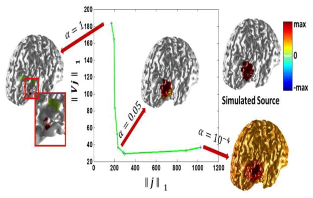
Fig. 2.

Selecting the hyper-parameter α using the L-curve technique. In order to select α which is a hyper-parameter balancing between the sparsity of the solution and gradient domain, the L-curve technique is adopted. As it can be seen a large value of α will encourage a sparse solution while a small value of α encourages a piecewise constant solution which is over-extended. The selected α needs to be a compromise. Looking at the curve it seems that an α corresponding to the knee is optimum as perturbing α will make either of the terms in the goal function grow and thus would not be optimal. The L-curve in this figure is obtained when a source with an average radius of 20 mm was simulated. The SNR of the simulated scalp potential is 20 dB.