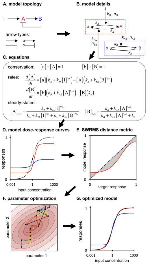
Figure 2.

Modeling scheme, illustrated by a two-node network with negative feedback. (A) Model topology; ‘I’ is the input, A and B are nodes, and arrows types depict interactions. (B) Detailed representation; dotted boxes are nodes, showing nominally inactive and active states and interconversion reactions, and black text symbols are model parameters. (C) Model equations; brackets denote concentrations of node species and the “s.s.” indicates steady-state. (D) Steady-state dose-response curves for the same model, using arbitrary parameters. The black dashed line is the target function, the red line is the node A response, and the blue line is the node B response. (E) SWRMS distance using the node A dose-response curve shown in panel D, now with the target response as the x-axis. (F) Parameter optimization. Brown ellipses show a contour graph of SWRMS distances near a minimum (small white circle). Four intermediate steps are shown in progressively warmer colors (blue, green, yellow, red) for each approach. Black dots mark the parameter estimates. Vertical and horizontal lines depict greedy random walk steps while triangles depict downhill simplex method steps. (G) Dose-response curves after optimization of model parameters for agreement with the target function.