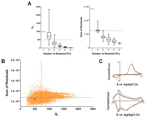
Figure 6.
Summary of “library” approach to generate randomized standard training sets. (A) Box plots showing the distribution of Qα threshold values (left) and the residual sum for all snippets (right) shown as a function of the number of PCs retained in the constructed PCR model. The values for the training set constructed within the experimental subject (subject B) are shown as a horizontal dashed lines. (B) Scatterplot showing the residual sums plotted against Qα values for all 2 PC models. The dashed lines correspond to the medians of the distributions in each variable. The model constructed with subject B’s training set is shown as a green square in the lower left quadrant. (C) Average kj vectors constructed from all 2 PC models (solid black line) and 2 PC models in falling in the lower half of the distributions for both the residual sum and Qα values (lower left quadrant of (B), dashed black line), as well as subject B’s PC model (orange dashed line).

