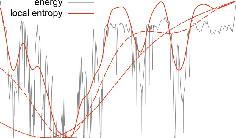
Fig. 1.

Energy landscape compared with local entropy landscape in an illustrative toy example. The energy landscape (gray curve) can be very rugged, with a large number of narrow local minima. Some isolated global minima can also be observed on the right. On the left, there is a region of denser minima that coalesce into a wide global optimum. The red curves show the local entropy landscape (Eq. 2 with the opposite sign) computed at increasing values of the interaction parameter $\gamma$ (i.e., at progressively finer scales). At low values of $\gamma$ (dashed curve), the landscape is extremely smooth and the dense region is identifiable on a coarse-grained scale. At intermediate values of $\gamma$ (dot-dashed curve) the global minimum is narrower and located in a denser region, but it does not correspond to a global energy minimum yet. At large values of $\gamma$ (solid curve) finer-grain features appear as several local minima, but the global minimum is now located inside a wide global optimum of the energy. As a consequence of this general picture, a process in which a local search algorithm driven by the local entropic landscape is run at increasing values of $\gamma$ will end up in such wide minima, even though in the limit $\gamma \to \mathrm{\infty }$ the local entropy landscape tends to the energy landscape. Note that in a high-dimensional space the isolated global minima can be exponentially more numerous and thus dominate the equilibrium measure, but they are “filtered out” in the local entropy description.