. 2016 Dec 7;5:e19695. doi: 10.7554/eLife.19695

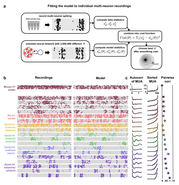
Figure 3. Deterministic spiking networks reproduce the dynamics observed in vivo.

(a) A schematic diagram illustrating how the parameters of the network model were fit to individual multi-neuron recordings. (b) Examples of spontaneous activity from different recordings, along with spontaneous activity generated by the model fit to each recording. (c) The left column shows the autocorrelation function of the MUA for each recording, plotted as in Figure 1. The black lines show the autocorrelation function measured from spontaneous activity generated by the model fit to each recording. The middle column shows the sorted MUA for each recording along with the corresponding model fit. The right column shows the mean pairwise correlations between the spiking activity of all pairs of neurons in each recording (after binning activity in 15 ms bins). The colored circles show the correlations measured from the recordings and the black open circles show the correlations measured from spontaneous activity generated by the model fit to each recording.

DOI: http://dx.doi.org/10.7554/eLife.19695.007

Figure 3.

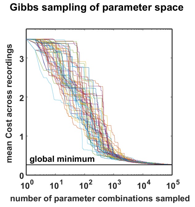
Figure 3—figure supplement 1. Optimization performance of the MCMC procedure.

Figure 3—figure supplement 1.

The total cost over all recordings is plotted as a function of sample number for 50 different optimizations, started with different random seeds. All the optimizations found near-global minima for all datasets with less than 100,000 samples. To efficiently conduct this analysis, we restricted the optimizations to the already fully-sampled grid, but the optimization procedure would in general allow sampling any parameter value by using a continuous instead of a discrete proposal distribution.
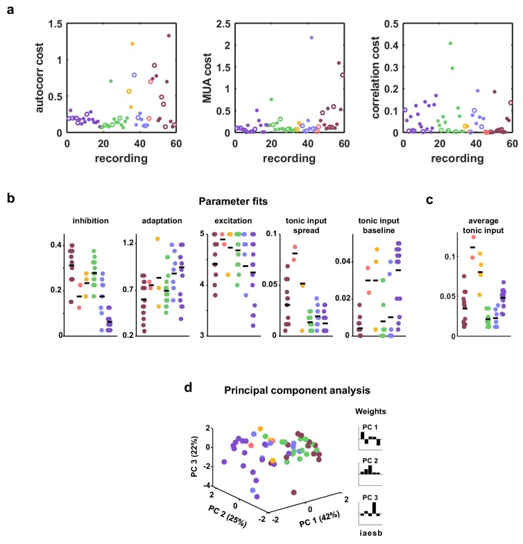
Figure 3—figure supplement 2. Costs and parameter fits.

Figure 3—figure supplement 2.

(a) The three separate terms that combine into our cost function are shown for each recording. Open circles indicate datasets shown in Figure 3. (b) All parameter fits for each recording. Colors are used to indicate recordings of the same type. A small jitter was added to the horizontal location of each point. Black lines indicate median values for each recording type. (c) The average tonic input in the network fit to each recording, computed as the sum of the baseline tonic input and the mean of the exponential distribution from which the random component of the tonic input for each neuron was drawn. To compare urethane desync and urethane sync parameter values, we used a Wilcoxon rank-sum test, and found the significance of the average tonic input in desync versus sync was p<102. The significance for adaptation, inhibition, excitation, and tonic input spread were p=0.491,p=0.236,p=0.349, and p=0.27, respectively. (d) A 3-dimensional principal component analysis shows that recordings generally cluster by type, but there is considerable variability both across and within recording types. The inset shows the 5-dimensional PCs.
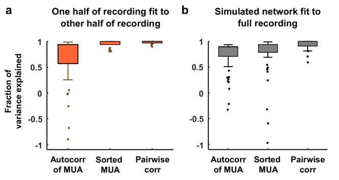
Figure 3—figure supplement 3. Variance explained by model fits.

Figure 3—figure supplement 3.

(a) Each neural recording was split into two halves (interleaved segments of 4 s each) and the autocorrelation function of the MUA, the distribution of MUA values across time bins, and the mean pairwise correlations were computed for each half. The fraction of the variance in the statistics of one half of each recording that was explained by the statistics of the other half of the recording is shown. The median variance explained for the autocorrelation function of the MUA, the distribution of MUA values across time bins, and the mean pairwise correlations were 84%, 98%, and 100% respectively. (b) The amount of variance in the statistics of each full recording that was explained by the model fit is shown. The median variance explained for the autocorrelation function of the MUA, the distribution of MUA values across time bins, and the mean pairwise correlations were 82%, 90%, and 97% respectively.
Figure 3—figure supplement 4. Analysis of local minima.

Figure 3—figure supplement 4.

Parameter identifiability has recently been raised as a potential problem in interpreting the results of network simulations. To mitigate this problem, we designed our model to have a very small number of parameters and we fit three different functions of the recordings, two of which varied as a function of time or rank. To confirm that the analysis of parameter combinations other than those corresponding to the global minimum of the cost function for each recording would not lead to a different interpretation of our results, we also considered local minima in regions of parameter space that were distant from the global minimum. It is possible that such local minima correspond to parameter regimes that are qualitatively different from the global minimum, yet still capture the statistics of the recordings relatively well. We found the parameters corresponding to local minima did not consistently emphasize the role of any parameter other than inhibition; the strength of inhibitory feedback remained the dominant influence on noise correlations, even for local minima far removed from the global minimum. (a) A schematic diagram showing an example nonlinear cost function. Several different threshold values are indicated by the colored lines. All costs below threshold are considered and the parameter q furthest away from the global minimum is chosen to plot in panel b. (b) As the threshold value is increased from the global minimum, the distance of the q with Cost (q) < threshold that is furthest from the global minimum is plotted. Discontinuities are visible when the threshold surpasses values at local minima. (c) Same as (b), but for the actual model fits to each recording. The values on the vertical axis are specified in terms of the grid spacing used for the Monte Carlo simulations. While some discontinuities are visible, the functions tend to increase gradually. (d) For each threshold value, we computed the r2 between the value of each of the five model parameters and noise correlations, as in Figure 5a. This analysis shows that considering local minima situated far from the global minimum serves only to diminish the relationship between inhibition and noise correlations, without revealing any strong relationships between noise correlations and any other parameter.