Figure 2.

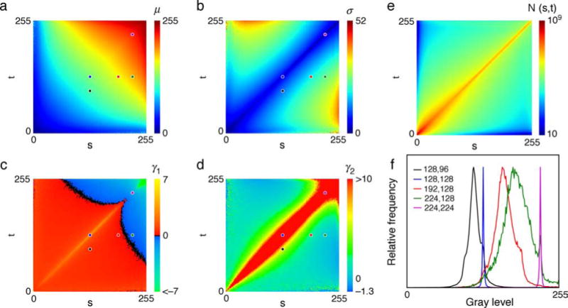
Conditional central moments for three neighboring image points. (a) The 1st moments are the means: μ = u₁. (b) The 2nd moments are plotted as the standard deviation: $\sigma =\sqrt{u_2}$. (c) The 3rd moments are plotted as the skewness: ${\gamma }_1=u_3/u_2^{3/2}$. (d) The 4th moments are plotted as the excess kurtosis: ${\gamma }_2=u_4/u_2^2-3$ (a Gaussian has an excess kurtosis of 0), where the central moments for each pair of values (s, t) were computed in the standard way: $u_1=n^{-1}{\displaystyle \sum x},u_2=n^{-1}{\displaystyle \sum {(x-u_1)}^2},u_3=n^{-1}{\displaystyle \sum {(x-u_1)}^3,u_4=n^{-1}{\displaystyle \sum {(x-u_1)}^4}}$ (see Kenny & Keeping, 1951; Papoulis, 1984). (e) Number of training samples for each value of s, t. (f) Conditional distributions for the five sample pairs of (s, t) values indicated by the dots in (a)–(d). The plots have not been smoothed.