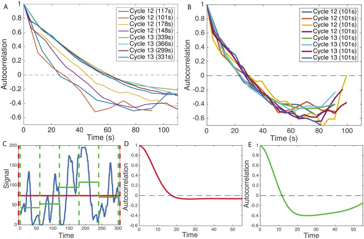
Fig 2. Autocorrelation analysis of fluorescent traces from cell cycles 12-13.

(A) Autocorrelation functions for traces of different length caused by the variable duration of the cell cycle. Each autocorrelation function is calculated from one embryo and one cell cycle from traces in the anterior region of the embryos. Reading off the autocorrelation time as the time at which the autocorrelation function decays by a value of e would give different values for each trace. The analysis is restricted to the steady state part of the traces (as defined in the text and S2 Fig). The durations of the steady state windows are given in SITable I. (B) Autocorrelation functions calculated for the same traces reduced to having equal trace lengths, all equal to the trace length of the shortest trace (101s), show that the differences observed in panel A are due to finite size effects. In the curtailed traces all sequential time points until the 101s time point were used. (C) An example of a signal simulated using the process described in Fig 1 for 300 seconds (blue curve) for a two state model. Taking the whole 300 second interval (red dashed lines) gives a good approximation of the average signal (red line) and the effect of finite size on the autocorrelation function is small (D). Reducing the time window to 60 seconds (green dashed lines) correlates the average with the signal much more and the effect of the finite size on the autocorrelation is strong (E). The sampling rates of the four embryos are: 13.1s, 10.2s, 5.1s and 4.3s, respectively. Parameters for the simulation in (C-E) are: k_on = k_off = 0.06s⁻¹, sampling time dt = 4s, for the red curve T = 300s and M = 2000 nuclei, for the green curve T = 60s and M = 10000 nuclei (same total amount of data). These parameters were chosen for illustrative purposes.