
Figure 1. Sequential establishment of chromatin accessibility at the MBT.
(A) (Left column) Single embryos were collected for ATAC seq at the indicated time points. Micrographs show stage-matched panels from a time-lapse image of a single Histone H2Av-GFP embryo. Scale bar = 10 μm. Coverage of sequence reads from accessible chromatin over the hunchback (center) and scylla (right) loci are shown. The hunchback P2 promoter/enhancer and associated shadow enhancer in addition to the later-acting stripe enhancer (arrows) are open and accessible at all time points measured. A schematic summarizing the regulatory interactions of the hunchback locus is shown at bottom left. The scylla TSS gains accessibility at NC12 + 9’ and is stably maintained thereafter. Scale bars (red) equal 1 kb. Plots show mean coverage from at least n = 3 replicates. (B) The fraction of each genomic feature present during each cell cycle is plotted as a stacked bar chart. ‘NC12 new’ and ‘NC13 new’ indicate the set of peaks newly called present in each respective cell cycle. Not shown: 2898 peaks not found to overlap with available genomic annotations used to classify enhancers, promoters, or insulators. (C) The association of functionally validated enhancers within each ATAC-seq timing class was calculated, and this plot shows what fraction of these are active at the indicated timepoints. Solid bars indicate the fraction of enhancers whose expression is first detected at the indicated timepoint. The lighter remaining bar indicates the total fraction of active enhancers associated with each ATAC-seq timing class. Color coding is as for panel B, and enhancers not overlapping with the ATAC-seq peaks are shown in red. The estimated elapsed time post NC11-NC13 for each scored stage of development (bottom axis) is indicated on the top axis. (D) Odds ratios for enrichment of the indicated genomic features and transcriptional regulators were calculated. Early chromatin accessibility is enriched for enhancers (p=2.54x10−109) and binding of Zelda (p=3.7x10−225). Late or dynamic chromatin accessibility is enriched for promoters (p=4.62x10−42), insulators (p=7.71x10⁻¹⁴), and binding of GAF (p=3.76x10⁻¹⁹). p-Values are from two-sided Fisher’s exact test on contingency tables constructed on [-/+ feature by early/dynamic].

Figure 1—figure supplement 1. Selection of metaphase-staged embryos and inter-replicate reproducibility.

Figure 1—figure supplement 2. Fraction of accessible peaks during metaphase.

Figure 1—figure supplement 3. Read-length distribution and comparison of interphase and metaphase library preparations.

Figure 1—figure supplement 4. Browser view of tribbles.
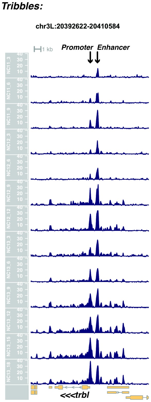
Figure 1—figure supplement 5. Browser view of empty spiracles.
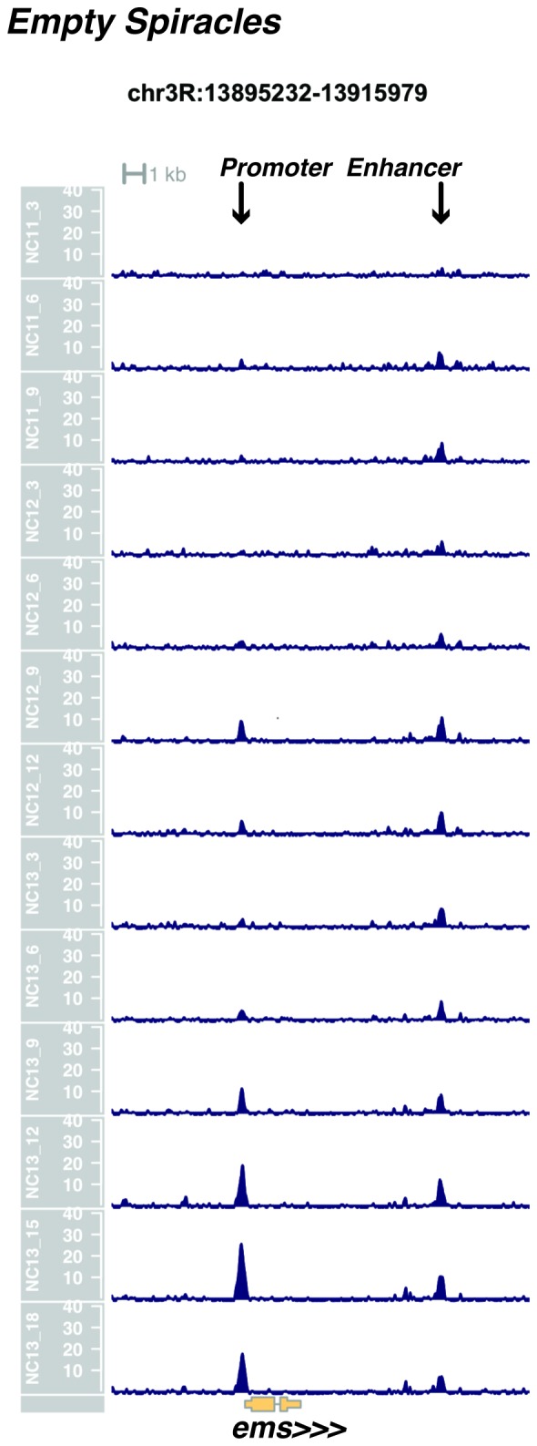
Figure 1—figure supplement 6. Browser view of Ultrabithorax.

Figure 1—figure supplement 7. Browser view of sloppy paired 2.
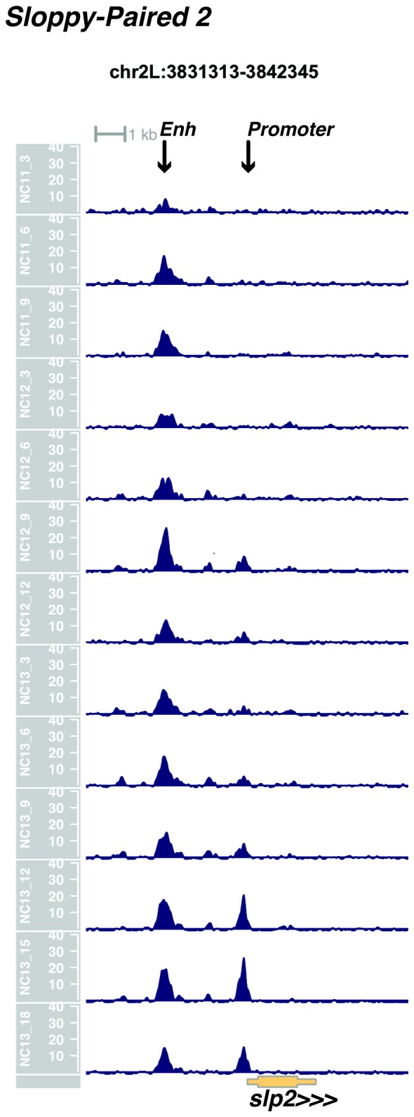
Figure 1—figure supplement 8. Browser view of forkhead.

Figure 1—figure supplement 9. Browser view of giant.

Figure 1—figure supplement 10. Browser view of Krüppel.
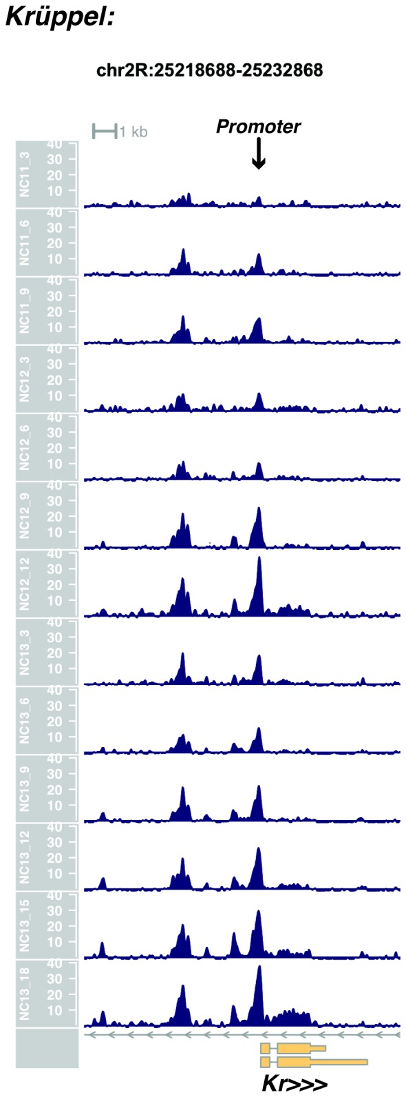
Figure 1—figure supplement 11. Browser view of knirps.
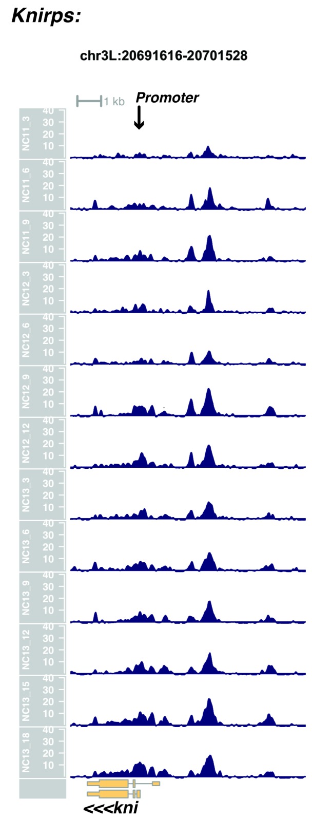
Figure 1—figure supplement 12. Browser view of even-skipped.
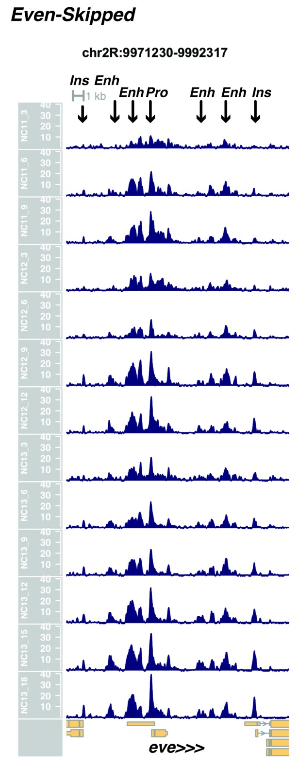
Figure 1—figure supplement 13. Browser view of hairy.
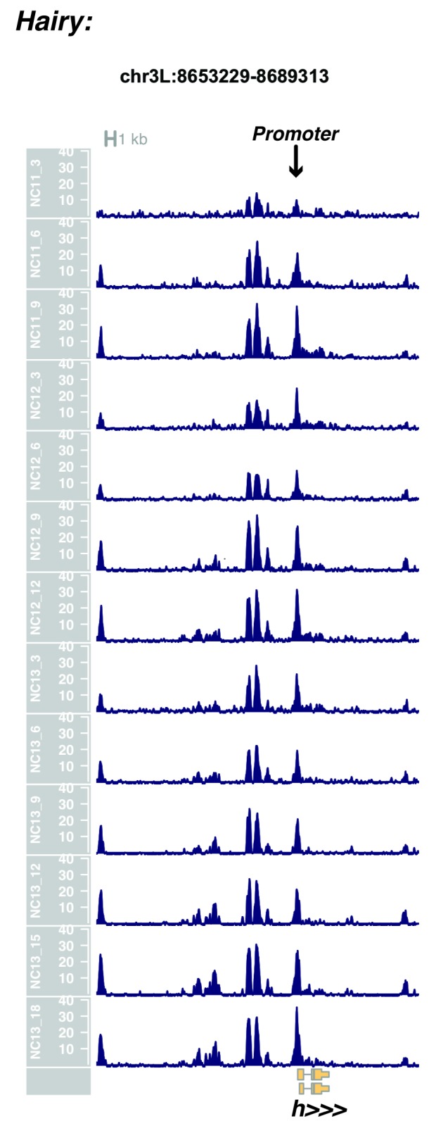
Figure 1—figure supplement 14. Browser view of odd-skipped.
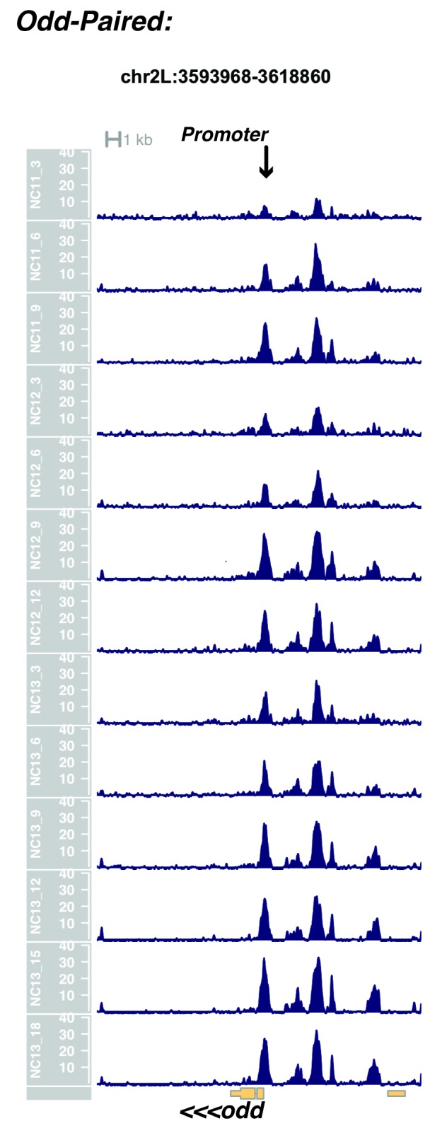
Figure 1—figure supplement 15. Browser view of fushi tarazu.
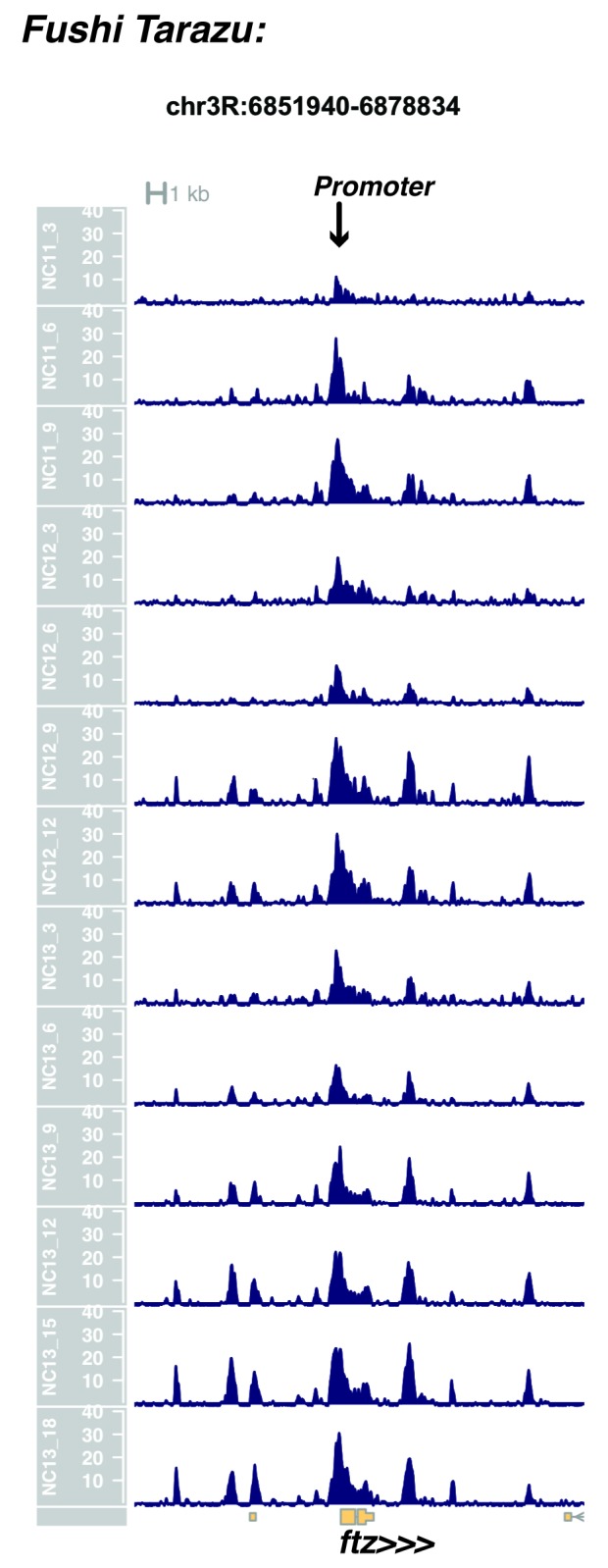
Figure 1—figure supplement 16. Browser view of runt.

Figure 1—figure supplement 17. Browser view of paired.

Figure 1—figure supplement 18. Browser view of sloppy paired 1.
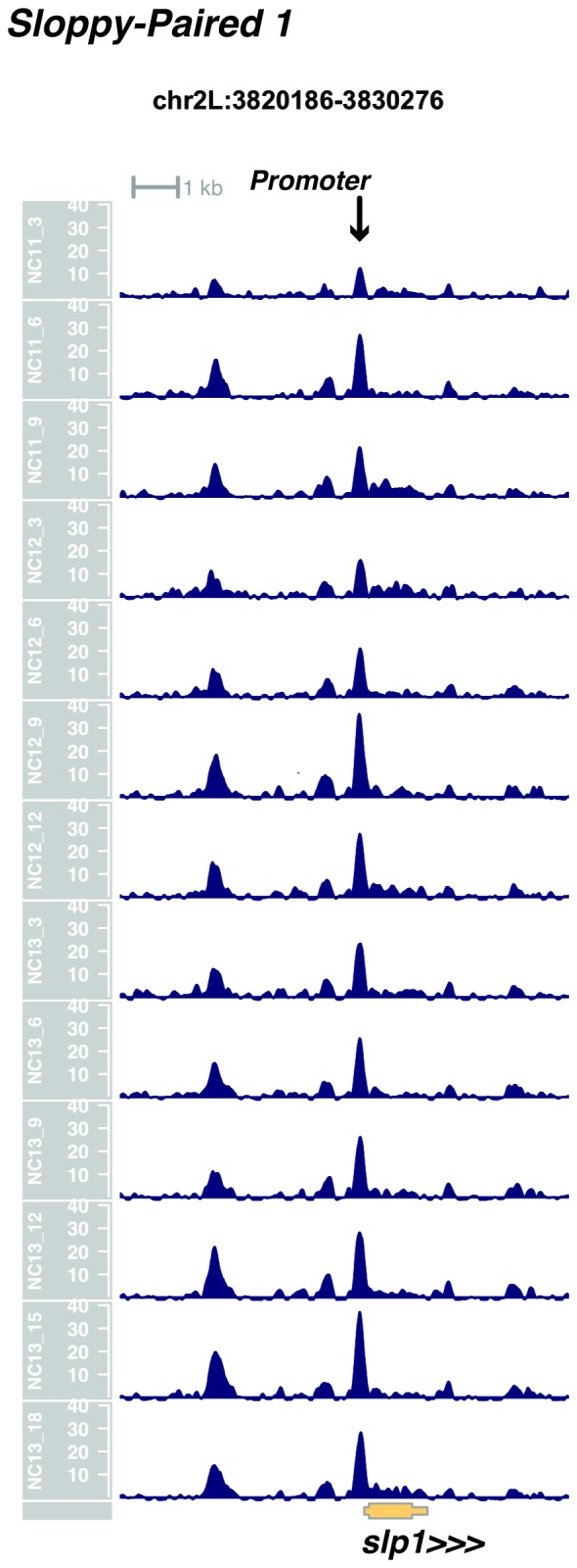
Figure 1—figure supplement 19. Browser view of odd-paired.
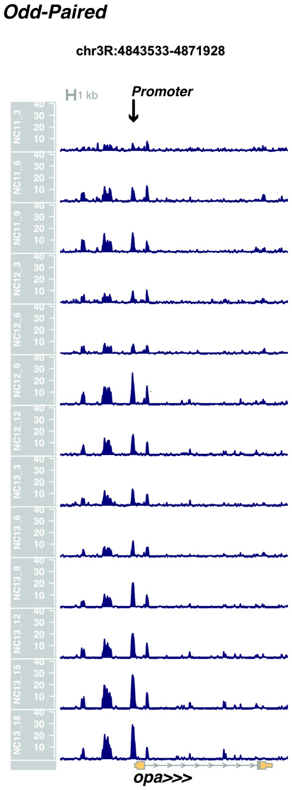
Figure 1—figure supplement 20. Browser view of huckebein.
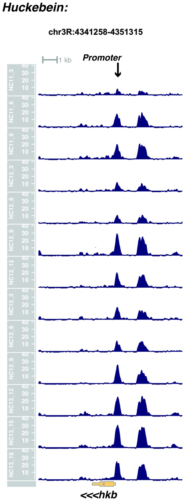
Figure 1—figure supplement 21. Browser view of tailless.
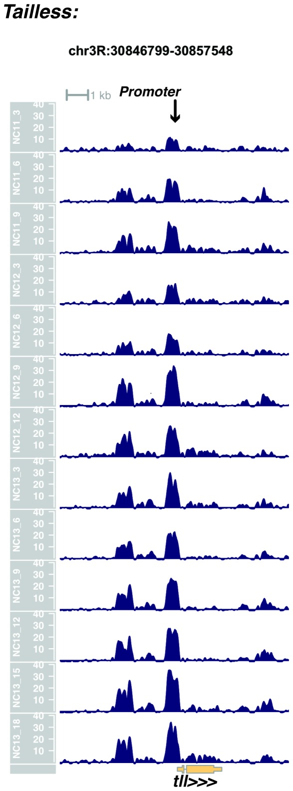
Figure 1—figure supplement 22. Browser view of wingless.

Figure 1—figure supplement 23. Browser view of engrailed.
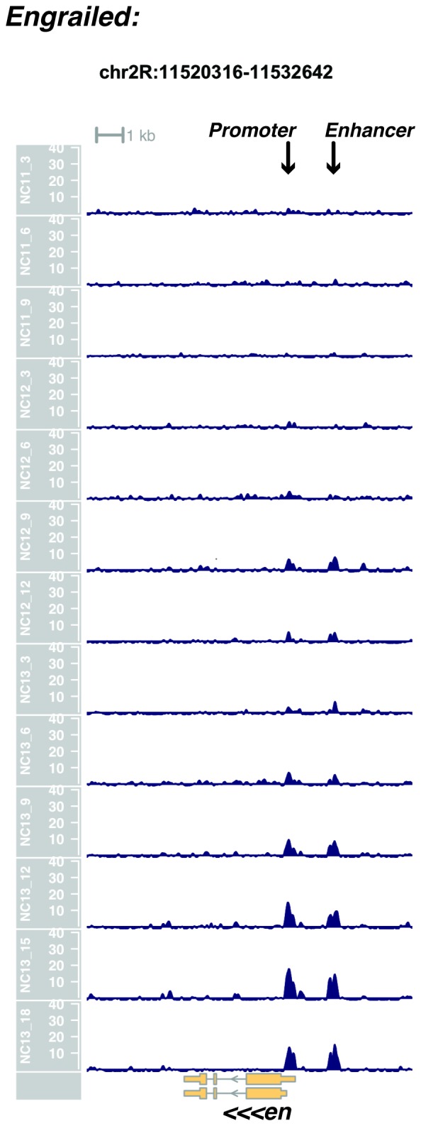
Figure 1—figure supplement 24. Browser view of patched.
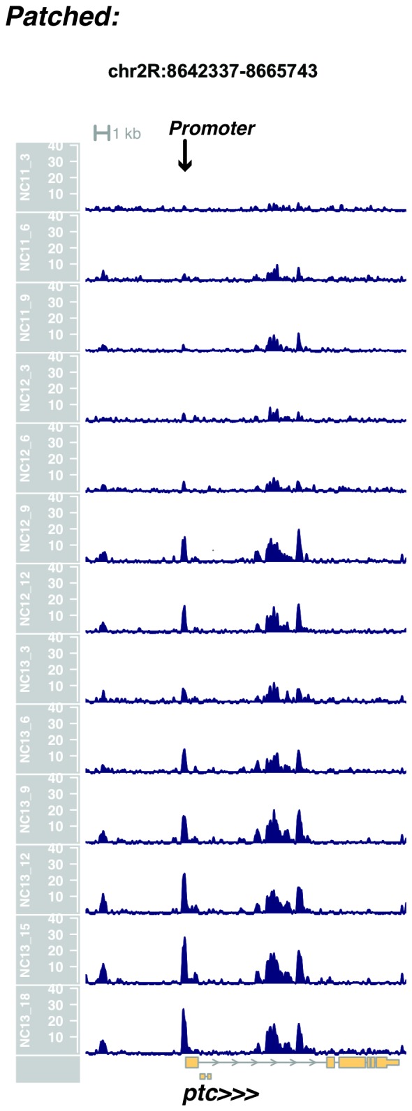
Figure 1—figure supplement 25. Browser view of hedgehog.
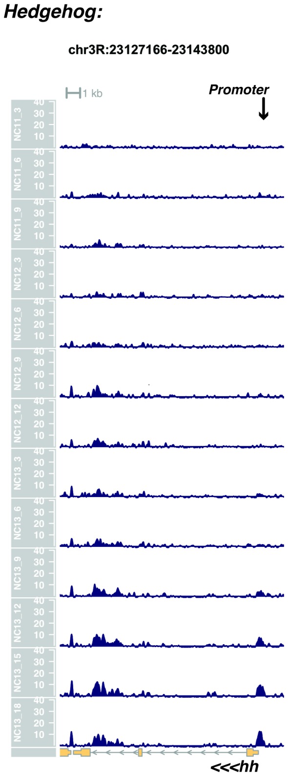
Figure 1—figure supplement 26. Browser view of crocodile.
