Figure 3. Patterns of stable and dynamic chromatin accessibility over the cell cycle.

(A) Genome-wide mean ATAC-open coverage is plotted (red, error bars show std. dev. between peaks, n = 9824) over the mean scaled heterogeneity in PCNA-EGFP to estimate DNA replication activity (blue, n = 4, error bars show std. dev. between embryos). Mitotic phases are indicated by grey shading. (B) Mean coverage of sequencing reads from accessible chromatin over the hunchback P2 promoter/enhancer is plotted (red) over the mean measured spot fluorescence intensity from a hunchback P2> MS2(24) LacZ: : MCP-GFP reporter (blue, n = 3, error bars show std. dev. between embryos). Mitotic phases are indicated by grey shading. (C) Immunofluorecence for chromatin morphology (DAPI) and RNA Polymerase II (CTD pSer5) in a region of an NC13 embryo transitioning from prophase to metaphase is shown. Observed mitotic states are indicated at left. Scale bar = 10 μm.

DOI: http://dx.doi.org/10.7554/eLife.20148.032

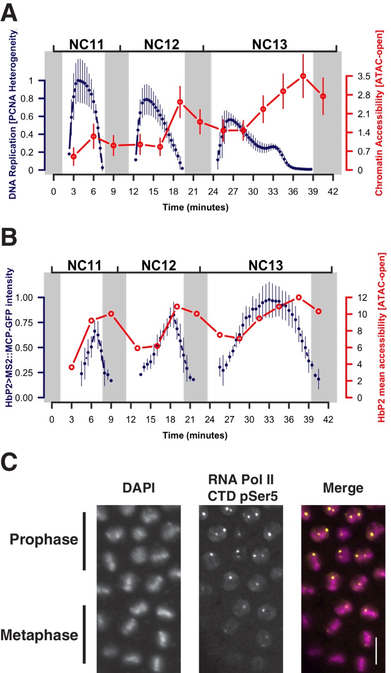
Figure 3—figure supplement 1. Example of PCNA-EGFP imaging and analysis.

Top panels show representative frames from one time-lapse image of a PCNA-EGFP embryo at the indicated timepoints during NC13. Note the distribution of brighter foci over time. Scale bar = 10 μm. An individual nucleus from each frame is enlarged and shown below to highlight the changing distribution of bright PCNA-EGFP over time. The bright foci correlate with the degree of DNA replication activity (see McCleland et al., 2009). To quantify the fraction of PCNA-EGFP fluorescent signal associated with heterogeneously distributed regions of fluorescence intensity, images were subjected to analysis as described in the Materials and methods. Measurement of the grayscale correlation matrix yields an estimate of homogeneity of neighboring pixel intensities within regions of interest (nuclei, scores range from 0 to 1 where 1 = all pixels neighbor pixels of similar intensity). We plot here the value of 1 - Homogeneity, where 0 = homogeneous neighbor intensities, and 1 = heterogeneous neighbor intensities. The timepoints corresponding to the shown representative frames are indicated by blue lines.

DOI: http://dx.doi.org/10.7554/eLife.20148.033