Figure 4.

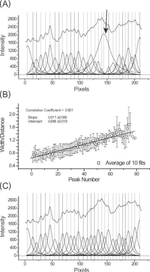
An overview of constrained peak fitting. (A) Shown are the results of an unconstrained peak-fitting session in which uniform peak widths were initially assigned. Note the variability of the peak widths far beyond the physically appropriate value in particular, the peak highlighted by the arrow. (B) The results of a calibration carried out using Equation 6 showing the linear relationship between peak number and peak width/inter-peak distances (). (C) The improvement resulting from the application of Equation 6 together with the peak width constraints that are described in the text. While correlation coefficients for panels A and C are 0.99981 and 0.99967, respectively, panel C accurately reflects the properties of the electrophoretic band separation.