Figure 4.

Quantification Based on Our Novel Modeling Approach

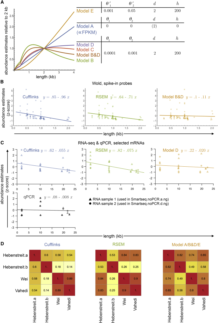
(A) Length dependency of abundance estimates for our models. The estimates are normalized to unity at length 2 kb. Parameter settings are shown in the table on the right.

(B) Abundance estimates for RNA spike-ins (ERCC-mix1) of the Wold dataset are plotted versus their lengths for three different bias-correction approaches (Cufflinks, blue; RSEM, green; our model B&D fit, orange). Each dot corresponds to one probe. Fitted trend lines and their formulas are shown. Standardized measures (Z scores) are used to make the approaches comparable.

(C) Abundance estimates for twelve randomly selected mRNAs (Table S2) covering a wide range of lengths. RNA-seq samples deriving from two different RNA samples (Table S1) were quantified by RSEM, Cufflinks, or our model D as indicated. In parallel, the corresponding two RNA samples (dots and triangle symbols, respectively) were subjected to qPCR for the same twelve genes. Presentation and analysis as in (B).

(D) Correlation matrices for abundance estimates of four datasets for the same cell type (resting Th2 cells) prepared with different library preparation protocols (Hebenstreit.a/b, random priming; Wei, poly-A tagging; Vahedi, RNA fragmentation). Different quantification approaches were used: Cufflinks (left panel), RSEM (middle panel), and our model fittings (Hebenstreit.a/b, model E; Wei, model B&D; Vahedi, model A). See Table 1 for details of the datasets.