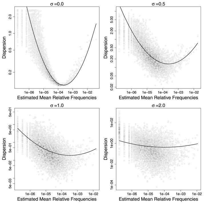
Figure 5.

As the noise level σ increases in the simulation model, the fitted dispersion model shows increasing lack of fit. In each plot above, the x-axis is the estimated mean relative frequencies, the solid curve corresponds to the fitted NBQ dispersion model, and black dots are the true dispersion values from the simulation model (see equations (6) and (7)). Note that when fitting the NBQ model (6), the true values of π_ij were unknown and needed to be replaced by the estimated values. The estimation errors in π_ij contributed to the estimation errors in the fitted dispersion model even when σ = 0.