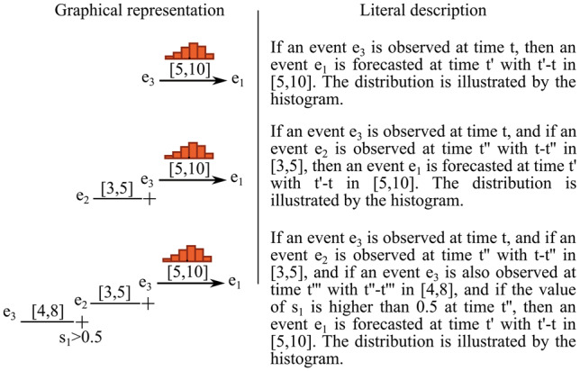
Figure 1.

Three examples of TITA rules: e1, e2, and e3 are generic events; s1 is a scalar and is assigned to a numerical value at each point in time. Histograms represent the probability distributions of the time difference between activation of the rule body and activation of the rule head. When the body of a rule is matched, the histogram is used to infer the probability distribution of the predicted event’s time of occurrence. Intervals between 2 events in the rule’s body define constraints on the time difference between the occurrences of these 2 events. Note that in this work, we focused on forecasting CRI events, therefore the head of the rules (ie, e1 events) will always be CRI.