

Abstract
We investigated the theoretical possibility of applying phenomenon of synchronization of coupled nonlinear oscillators to control alternate bearing in citrus. The alternate bearing of fruit crops is a phenomenon in which a year of heavy yield is followed by an extremely light one. This phenomenon has been modeled previously by the resource budget model, which describes a typical nonlinear oscillator of the tent map type. We have demonstrated how direct coupling, which could be practically realized through grafting, contributes to the nonlinear dynamics of alternate bearing, especially phase synchronization. Our results show enhancement of out-of-phase synchronization in production, which depends on initial conditions obtained under the given system parameters. Based on these numerical experiments, we propose a new method to control alternate bearing, say in citrus, thereby enabling stable fruit production. The feasibility of validating the current results through field experimentation is also discussed.
Alternate bearing (biennial bearing) is a common phenomenon in many tree crops, in which a year of heavy crop yield, known as the “on-year” is followed by an “off-year” of extremely light or no yield1,2. This pattern continues in subsequent years. Synchronization of fruit production observed in orchards and national markets is also called alternate bearing. Alternate bearing in individual trees and orchards is a challenge for farmers because they need advanced skills to maintain constant production3. Farmers and agronomists have recognized alternate bearing of tree crops as a complex phenomenon, and various efforts have been made to understand its behavior and mechanisms4.
Similar to alternate bearing, the phenomenon of acorn masting has been a common subject in studies of forest and ecological management5,6,7,8,9. Isagi10 was the first to develop a simple nonlinear dynamics model to explain the annual oscillations of acorn production in an individual tree. This model is called the resource budget model (RBM) because it is based on the energy (photosynthate) stored in a plant. Isagi also attempted to explain the synchronization of acorn production in a large population (i.e. masting) by globally coupled RBM oscillators. This coupling is mainly caused by pollination in oak trees.
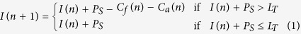
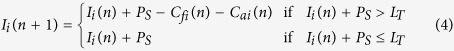
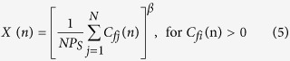
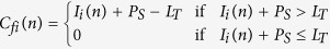
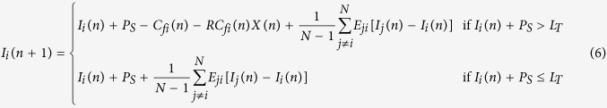
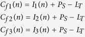
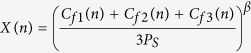
The RBM model is based on the amount of photosynthate produced each year in an individual plant. The majority of photosynthate is used for the plant’s growth and maintenance. The remaining photosynthate (Ps) is stored in the plant. The accumulated photosynthate stored in a plant is expressed as I. In a year when accumulated photosynthate exceeds a certain threshold LT, then the remaining amount, I – LT, is used to represent the cost of flowering, Cf. These flowers are then pollinated and bear fruit, the cost of which is designated as Ca. Usually, the fruiting cost is a function of the cost of flowering, i.e., Ca = F(Cf) where F(.) is a function. The accumulated photosynthate becomes I = LT after flowering. Once fruiting is over, the remaining photosynthate becomes LT−Ca i.e., I = LT − F(Cf). In the RBM, we consider the function F(Cf) to be linear, i.e., Ca = R Cf where R is a proportionality constant that represents the flowering to fruiting ratio. In this case, the phenomenon is modeled as10,11,12,13,14,15.
 |
 |
where n = 1, 2, 3…. represents the years. Here R is considered as a control parameter for this model. Figure 1 shows a bifurcation diagram, I, as a function of the parameter R. At lower values of R < 1 (in region A1) there is only a single stable solution (Period-1 regime:A1, shown by the solid red line), indicating constant yields across years (i.e., no alternate bearing occurs). As R exceeds 1, the fixed point solution becomes unstable. Here, the upper and lower chaotic bands, which individually have an infinite number of bands16, correspond to high and low yields respectively (Multi-band chaotic regime:A2).
Figure 1. Bifurcation diagram, I, showing a function of parameter R, for the single-resource budget model,Eq. (1).
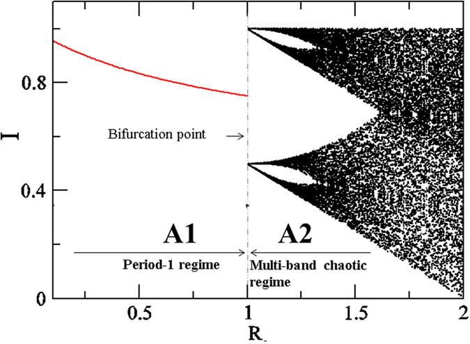
Regions A1 and A2 correspond to period-1 regime and multi-band chaotic regime, respectively16.
The RBM has been employed to explain the alternate bearing of Citrus unshiu, which is a parthenocarpicy species. Sakai17 validated a one-year forward prediction using and an experimental dataset and also applied the nonlinear control theory18 to estimate the control input needed to suppress alternate bearing19. Recently, some of the dynamical properties of this phenomenon have been uncovered using this model16. Attempts to let RBM fit the real behavior of C. unshiu have been carried out using experimental data20.
The conventional method of producing C. unshiu fruit aims to stabilize output by fruit thinning and pruning. In terms of nonlinear dynamics, this can be thought of as stabilizing the state (i.e., fruit production volume) at an unstable fixed point. Therefore, we can think of the conventional production method as equivalent to controlling chaos, similar to the OGY method18; though farmers and agronomists surely carry out these procedures based on empirical observations rather than the underlying theory. However, this conventional method still requires farmers to have very advanced skills to be able to determine the appropriate amounts of fruits and/or flowers to remove3.
The main objective of this paper is to propose a new fruits production method to get constant total fruits production form an orchard of Citrus unshiui by enhancing alternate bearing of individual citrus trees, based on the principles of phase synchronization of coupled oscillators and utilizing the existing RBM10,12,13,14,21. We propose a production method using direct coupling between citrus trees. In practice, two is the appropriate number of connected trees. Our method (the direct coupling method) aims to realize artificial alternate bearing by grafting two (or more) trees. In a given orchard with N trees, this method incorporates the fact that N/2 trees are experiencing an on-year and the rest an off-year at any given time, which allows the total production of N trees to be constant every year22.
We have organized this paper as follows: Section II discusses the interactions between plants under different types of coupling. Section III offers the results for two and three coupled plants. Section IV highlights the feasibility of experimentation. Section V summarizes the results.
Modeling Plant Interactions
In a real-world plant population, many types of interactions occur among plants, resulting in various types of dynamic behaviors23,24. Synchronization is one such phenomenon that occurs as a result of interactions between systems. Synchronization happens when plants’ actions are in unison i.e., when their subsystems follow the same life cycle schedule25,26. This behavior has been well studied and has been found to be present in almost all branches of science13,26,27, including in ecology28,29,30,31,32. Many types of synchronization, such as complete, lag, intermittent, and generalized synchronization27, have been observed as a result of interactions between systems. These have been discussed in detail in the literature27. Phase synchronization27,33 is one such type of synchronization, in which the amplitudes of individual oscillators (e.g. plants) are uncorrelated, while their phase-difference remains bounded. If the phase-difference of the oscillators is near zero, then it is termed “in-phase” behavior. If the phase-difference is near π, then it is called “out-of-phase” behavior26,33,34,35,36,37. In this work, we also explore the possibility of in- and out-of-phase behaviors among plants in the presence of different types of interactions. The models for three types of interactions, indirect, direct and mixed coupling, are discussed below (Fig. 2(a) and (b)). Here, the main target plant is a Citrus species. As Citrus unshiu is parthenocarpic, the effect of pollen coupling is much smaller than in cross-pollinating species, such as Citrus hassaku. Therefore, we took C. unshiu as the target for our direct coupling model and C. hassaku for the indirect coupling model. If a C. unshui orchard were located near to a C. hassaku orchard, the C. unshui would cross-pollinate and produce seeded fruits from the C. hassaku pollen. In other words, the indirect couplings shown in Fig. 2(a) and (b) model the effect of cross-pollination of Citrus hassaku.
Figure 2. Schematic drawing and real images for interactions.

(a) Two plants and (b) three plants. The solid and dashed arrows indicate direct and indirect interactions, respectively. The representative photographs show direct coupling between (c) the trunks/branches of Crape myrtle (Lagerstroemia indica) (source: Professor Tsuneo Ogata) and (d) the roots of three Pseudoacacia (Robinia pseudoacacia) trees.
Direct interaction (diffusive coupling): grafting
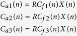
Grafting is an important technique by which plant parts (e.g. branches) are taken from one or more different plants and joined to another plant, the rootstock. Although grafting is a very popular technique, to our knowledge, it has not been used thus far in alternate-bearing plants to control the production. Recently, the joint tree training technique37,38 was developed to decrease the labor needed for tree training (e.g. brunching, thinning and pruning) of deciduous broad-leaved fruit trees such as pear, peach and apple. The joint tree training technique involves connecting trees along a line by grafting neighboring trees together. As the alternate-bearing in deciduous broad-leaved fruit trees is weaker than in Citrus spp.(evergreen trees), the joint training technique does not aim to control alternate bearing of them. Trees can also exhibit natural connections through branches, trunks, and roots39,40. Figure 2(c) and (d) show representative connections between branches/trunks and roots for different trees, respectively. These are typical examples of the natural physiological integration of plants; this type of interaction is referred to as “direct coupling” in this paper. In this work, we place emphasis on this type of integration and try to understand alternate-bearing behaviors in the presence of direct coupling. Direct coupling should realize physiological integration so that diffusive energy transfer can occur between the coupled plants. Hence, we can describe the direct coupling model as diffusive coupled nonlinear oscillators in eq. (3).
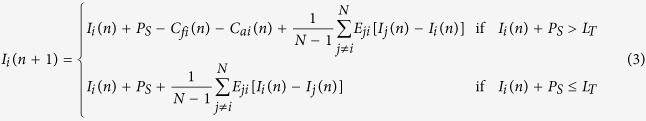 |
Here,  ,where Eji is the coupling strength for the direct interaction between the jth and ith plants. We consider that Eji = ε in Eq. (3) for simplicity. This coupling is illustrated as solid black arrows in Fig. 2(a,b) between different plants (circles).
Indirect interaction (mean-filed coupling): pollination
Plants interact with each other via external agents that can be biotic (e.g., animals, birds, fungi or bacteria) or abiotic (e.g., water, light, wind, soil, humidity or gases). Indirect coupling has been well studied in ecology and has been shown to affect plant populations in many ways. For example, pollen interactions with wind and insects enhance seed and/or fruit production in plants5,6,7,13,41,42,43,44.
The indirect coupled RBM model is expressed
 |
Here, 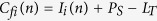 and
and 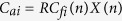 (cf. Eq. (2)). where
 |
 |
Mixed interaction: direct and indirect
In this paper, we consider two types of mixed interactions as illustrated in Fig. 2(a) and (b). Figure 2(a) is the interaction of two trees coupled directly and indirectly. Figure 2(b) is a network of three oscillators (plans), in which two plants have direct interaction in addition to the indirect interaction among all three plants. This can be demonstrated by combining Eqs (3) and (5). The mixed interaction models the case in which the orchard of Citrus unishiu is located near to a C. hassaku orchard.
 |
Results and Discussion
Effects of direct and indirect interactions in two coupled plants
To show the effect of both types of coupling we first consider two coupled plants (Fig. 2(a)) in the presence of either direct or indirect interactions in the period-1 regime (A1) and multi-band chaotic regime (A2), as alternate bearing is supposed to occur mostly in these two regimes according to experimentally estimated R values11.
Period-1 regime, A1: R = 0.5
To demonstrate the function of direct interaction (coupling), we first consider the period-1 regime R < 1 (marked as A1 in Fig. 1) because the conventional RBM does not generate any oscillation in the range of R < 1. Note that R = 1 is the only clear bifurcation point of the conventional RBM.
Period-2 bifurcates from period-1 at ε = 0.25 as shown in Fig. 3(b). This is a characteristic property of directly coupling two RBMs (single oscillators). In region P2, ε ≥ 0.25, we find out-of-phase behavior, as shown in Fig. 3(c) at ε = 0.4. In A1 (R < 1), this out-of-phase behavior occurs for any initial conditions. Figure 3(d) shows the normalized fractions of the initial conditions for either in-phase (fin) or out-of-phase (fout). These fractions are calculated as follows. If  , then both plants show out-of-phase behavior; otherwise they display in-phase behavior. We considered 1000 random initial conditions in I1∈[0, 1] and I2∈[0, 1], and we determined whether they would result in in-phase behavior (fin) or out-of-phase behavior (fout). Figure 3(d) clearly shows that fin is zero while fout is 1.0, which indicates that the plants produce fruits in an out-of-phase manner. This suggests that, with direct coupling, plants can be switched to an out-of-phase mode of fruit production even under Period-1 regime (A1) shown in Fig. 1.
Figure 3. Coupling at Peridod-1 regime: R = 0.5.
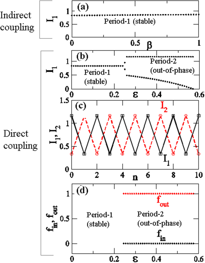
(a) The bifurcation diagram, I1, with the function of indirect (pollen) coupling strength β. For direct coupling: (b) the bifurcation, I1, as a function of coupling strength ε. (c) the trajectories of individual plants with time at coupling strength, ε = 0.4 and (d) the normalized fraction initial conditions with the function of coupling strength ε.
Multi-band chaotic regime, A2: R = 1.2
To show the dynamics of two coupled plants when they are in a multi-band chaotic regime (A2) in Fig. 1, we considered that R = 1.2. This value is very close to that estimated using experimental data for C. unshiu yield11. At this parameter value (R = 1.2), there are many chaotic bands; however these are separated in two parts: above and below the unstable period-1 fixed point16. At R = 1.2, individual plants show alternate bearing that appears cyclic (i.e., with “on-years” followed by“off-years”). However, the precise fruit-bearing behaviors are actually chaotic. The results for coupled plants when R = 1.2 are shown in Figs 4 and 5 for direct and indirect couplings, respectively.
Figure 4. Direct coupling at multi-band chaotic regime, A2: R = 1.2.

(a) The bifurcation diagram, I1, and (b) the fraction of the initial conditions corresponding to the in-phase (fin -line) and out-of-phase (fout -line) states as a function of ε. (c) The basins for the initial conditions for the in-phase and out-of-phase states are shown in black and red regions, respectively. The trajectories, I1 and I2, for coexisting (d) in-phase and (e) out-of-phase attractors at ε = 0.1 are shown.
Figure 5. Indirect coupling at Peridod-2 regime: R = 1.2.

(a) The bifurcation diagram, I1, and (b) the fraction of the initial conditions corresponding to the in-phase (fin -line) and out-of-phase (fout -line) states as a function of β. (c) The basins for the initial conditions for the in-phase and out-of-phase states are shown in black and red regions, respectively. The trajectories, I1 and I2, for coexisting (d) in-phase and (e) out-of-phase attractors at β = 0.1 are shown.
Direct coupling RBM
Here, we discuss the dynamic behavior of direct coupling RBMs. The results of direct coupling are shown in Fig. 4. The bifurcation diagram, Fig. 4(a), shows that multi-band chaos starts merging and becomes single-band chaos at approximately ε = 0.25. The fractions of the initial conditions (Fig. 4(b)) show that there is always an increase in out-of-phase motion as coupling strength ε is increased (i.e. direct coupling induces out-of-phase motion at higher coupling strengths ε). However, within this given parameter range, both in- and out-of-phase behaviors coexist. Figure 4(c) shows the basins of these coexisting attractors, in- and out-of-phase, in black and red, respectively, at ε = 0.1. The typical trajectories of in-and out-of-phase behaviors are shown in Fig. 4(d) and (e), respectively, at ε = 0.1. For the alternate bearing of C. unshiu, we hypothesize that pollen coupling will have little effect because the species is parthenocarpic. Therefore, the results obtained here are very useful for developing an improved method for producing C. unshiu fruits. In conventional citrus production, citrus trees are never joined by grafting or other methods. Therefore, the ratio of in-phase to out-of-phase trees is 1:1 as we can see in Fig. 4(b) at ε = 0. The strength of direct coupling ε should be estimated in field experiments. Physiological integration is expected when grafting two citrus trees. Thus, we expect to realize a positive value of ε in field experiments.
Indirect coupling RBM
Figure 5(a) shows the bifurcation diagram of I1 with the control parameter β, which demonstrates that multi-band chaos continues to exist; however, periodic windows occur in between. Figure 5(b) shows the fractions of out-of-phase and in-phase states with fout and fin. Note that owing to indirect interaction (pollen), we only obtain an in-phase solution after β = 0.25, which indicates that indirect coupling induces in-phase behavior at higher coupling strengths. Below β = 0.25, we obtain coexisting attractors. Figure 5(c) shows the basins of these coexisting attractors at β = 0.1, where the black and red regions show the initial conditions leading to the in-phase and out-of-phase states, respectively. Figure 5(d) and (e) show the typical trajectories for coexisting in-phase and out-of-phase attractors, respectively, at β = 0.1.
Effect of mixed interactions in two plants
In the previous subsections we considered the effects of direct and indirect coupling separately. Now we consider the simultaneous presence of both these interactions in two coupled plants (Fig. 2(a)) for R = 0.5 (Period-1 regime:A1) and 1.2 (Multi-band chaotic regime, A2). The results are shown in Fig. 6 (a) and (b) at R = 0.5 and 1.2, respectively, in the plane β−ε. The contour in Fig. 6(a) illustrates the critical line (between red and black) where period-1 bifurcates into period-2. The line corresponds to the largest Lyapunov exponents (LLE) at zero45. This shows that in region P2 the behaviors of both the plants are out-of-phase (fout > 0.8, similar to Fig. 3(b)). Figure 6(b) illustrates the contours map of fout from 0.1 to 0.8. This shows that out-of-phase behavior is enhanced as direct coupling strength, ε, increases. Figure 6(a) and (b) confirm that out-of-phase behavior can exist in the presence of both types of interactions and that it increases with increasing ε. This implies that direct coupling induces out-of-phase behavior even under indirect interactions.
Figure 6. Two plants coupling: Schematic phase diagrams in parameters space, β -ε.

(a) At R = 0.5 and (b) R = 1.2. P1 and P2 in (a) correspond to period-1 and 2 respectively. 5 Regions are demarcated after considering the contour on fraction of initial conditions leading to out-of-phase synchronized motions at 0.1 to 0.80.
Effect of mixed interactions in extended systems
Indirect interactions are a global phenomenon, affecting all elements in the systems in the same way. For example, in a given orchard, an external agent such as airborne pollen will affect all flowering plants equally (Eq.(4)). Figure 2(b) represents this example for three coupled plants, where pollen interactions (dashed line, β ≠ 0) exist between all the plants. In contrast, direct coupling is a local factor, and its interactions depend on the plants selected. Practically, it is almost impossible to couple all the plants in a system by grafting them together. To visualize the effects of direct coupling (in a few plants) and indirect coupling (in all available plants) in an orchard with many plants, we present a model for three representative, coupled plants, as in Fig. 2(b). Here, direct coupling exists only between two plants, while indirect coupling is present for all the plants. The dynamical model for this system becomes
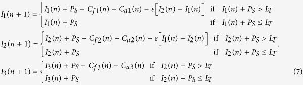 |
 |
 |
 |
The results are shown in Fig. 7 (a) and (b) for R = 0.5 and R = 1.2, respectively. The different regions are marked as those in Fig. 6 for the first and the second plant. The results clearly show that direct coupling induces iut-of-phase synchronization as well as in Fig. 6.
Figure 7. Three plants coupling: Schematic phase diagrams in parameters space, β -ε.

(a) at R = 0.5 and (b) R = 1.2 for coupled three plants, model Fig. 2(b), in the presence of mixed interactions, Eq. (7). 5 Regions are demarcated after considering the contour on fraction of initial conditions leading to out-of-phase synchronized motions at 0.1 to 0.80.
Comparisons of the figures for two (Fig. 6) and three oscillators (Fig. 7) confirm that the out-of-phase behavior between plants can be dominant and persistent in significant range of the β -ε space. This also indicates that, in a given orchard, direct coupling should be able to induce out-of-phase behavior between directly coupled plants by setting appropriate initial conditions of two coupled trees to be out-of-phase. Note that the calculation in Figs 6 and 7 were carried out to a maximum of ε = 1, although the ecologically meaningful range may only reach the lower values seen in Figs 3 and 4.
Experimental feasibility
In this section, we discuss the possibility of verifying the theoretical data obtained from modeling through field experiments and the potential limitations on such studies. Figure 3(d) shows that direct coupling induces out-of-phase behavior even in the period-1 regime (A1 region). Similarly Fig. 4(b) also suggests that the fraction of out-of-phase behavior is dominant for chaotic coupled behaviors. This out-of-phase dominance also persists in the presence of both types of interactions, as shown in Figs 6 and 7 for two and three coupled plants, respectively.
As these results show a higher likelihood of out-of-phase behavior occurring in the presence of both indirect interaction types, we may be able to use this property to control yearly fruit production. Let us suppose that we have N plants in a given orchard. If we are able to directly couple only N/2 pairs of plants (a single plant is directly connected to only one other plant), then we can control the total production of the orchard. That is, half of the plants will be in an “on-year” while the remaining half will be in an “off-year” owing to the dominance of out-of-phase dynamics. Therefore, the total production of the orchard across years will remain constant. Note that this strategy does not change the underlying action of alternate bearing, but it facilitates uniform production (shifting the fruit bearing timing of paired plants) by allowing only half of the plants to undergo fruit bearing in a given year.
Another very important observation can be drawn from Fig. 3 as follows. Suppose we wish to have constant production in just two plants. Let us achieve constant output in the uncoupled plants (as in regime A1 in Fig. 1) by proper thinning method46. If we are able to directly couple these plants, then we can expect out-of-phase production only for these plants, as shown in Fig. 3(b), at higher direct coupling strengths. This means that we can achieve constant output each year. This will result in a situation (as in Fig. 3(b)) in which we only obtain out-of-phase behavior at higher coupling strengths even in Period-1 regime(A1:R < 1). It is a remarkable advantage as a fruit production method for alternate bearing tree crops.
Therefore, we suggest that this direct coupling method can be used to achieve constant total production of an orchard. One limitation facing experimental validation of this theory is the presence of coexisting in- and out-of-phase behaviors depending on their initial conditions, as shown in Figs 4(c) and 5(c). Because plants are affected by external factors, there is the possibility of either starting from the basin of in-phase behavior or switching between in- and out-of-phase behaviors. Importantly, as we see in Figs 4(c) and 5(c), the basin boundaries are smooth (i.e., the boundaries are not as complex as riddled47,48,49 or fractal ones) therefore known controller techniques50 and we can easily set the initial conditions for the out-of-phase state. If an appropriate and feasible technique for basin switching/control is designed, then direct coupling could be very useful. Thus, we propose here that direct coupling may be useful for future stable fruit production. We hope the theoretical results presented will stimulate initiatives to develop future applications for controlling constant fruit production.
Summary
Considering the potential importance of ensuring constant fruit production in alternate-bearing plants, here we propose a theoretical concept based on nonlinear dynamics for controlling fruits production. We utilized the existing RBM, which captures many of the alternate-bearing plant phenomena. We coupled plants directly by grafting, which enhanced out-of-phase among plants. These directly coupled plants showed dominant out-of-phase synchronization, even in the presence of indirect interactions (e.g., pollen), suggesting the possibility of controlling fruit production. We show that once plants are directly coupled, it is possible to control plant behavior without further manual interference. That is, the proposed technique is automatic and self-sustaining. In this work, we offer the models for two and three coupled plants in the presence/absence of direct and indirect interactions. These models had similar results, suggesting that the conclusions presented here would likely apply to orchards with many plants. We have utilized one well-known model that captures many properties of the alternate-bearing phenomenon. However other variants of this model, such as those described in other studies15,46,47, could be considered for generalizing the presented results. Verifying the theoretical results presented here through field experiments is possible, but will take many years, perhaps decades. Above we have discussed the feasibility and potential limitations of field studies. We believe this initial proposal for controlling production in alternate-bearing plants could serve as a basis for further development of this concept.
Additional Information
How to cite this article: Prasad, A. et al. Direct coupling: a possible strategy to control fruit production in alternate bearing. Sci. Rep. 7, 39890; doi: 10.1038/srep39890 (2017).
Publisher's note: Springer Nature remains neutral with regard to jurisdictional claims in published maps and institutional affiliations.
Acknowledgments
A.P. received support from the Japan Society for the Promotion of Science (JSPS) through an invited fellowship (S-15093) to visit the Tokyo University of Agriculture and Technology, Tokyo, Japan, where this work was initiated. The Department of Science and Technology of Indian Government also provided financial support. K.S. appreciates support from JSPS grants-in-aid Nos. 1938014, 25660204, and 15KT0112. The authors thank Professor Tsuneo Ogata at Kochi University, Japan for permitting us to use the photograph in Fig. 2(c) and Dr. Takuya Ban of the Tokyo University of Agriculture and Technology, Japan for his technical advice about joint tree training. The authors appreciate the constructive comments of the anonymous reviewers.
Footnotes
Author Contributions A.P. conceived of the research and developed the model. A.P. and K.S. both conducted the numerical simulations, the analysis of the results and manuscript writing. Y.H. participated in the discussions and provided valuable suggestions.
References
- Monselise S. P. & Goldschmidt E. E. Alternate bearing in fruit trees: A review. Horticulture Review 4, 128–173 (2011). [Google Scholar]
- Goldschmidt E. E. The evolution of fruit tree productivity: a review, Economic Botany 67, 51–62 (2013). [DOI] [PMC free article] [PubMed] [Google Scholar]
- Meland M. Effects of different crop loads and thinning times on yield, fruit quality, and return bloom in Malus×domestica Borkh. ‘Elstar’. Journal of Horticultural Science & Biotechnology ISAFRUIT Special Issue 117–121 (2009). [Google Scholar]
- Shalom L. et al. Alternate Bearing in Citrus: Changes in the Expression of Flowering Control Genes and in Global Gene Expression in ON- versus OFF-Crop Trees. PLOS ONE 7(10), e46930 (2012). [DOI] [PMC free article] [PubMed] [Google Scholar]
- Koenig W. D. & Knopes J. M. H. The mystery of masting in trees. American Scientist 93, 340–347 (2005). [Google Scholar]
- Koenig W. D., Knopes M. H., Carmen W. J. & Pearse I. S. What drives masting? The phenological synchrony hypothesis. Ecology 96, 184–192 (2015). [DOI] [PubMed] [Google Scholar]
- Kelly D. & Sork V. L. Mast seeding in perennial plants: why, how, where? Annu. Rev. Ecol. Syst. 33, 427–447 (2002). [Google Scholar]
- Satake A., Bjrnstad O. N. & Kobro S. Masting and trophic cascades: interplay between rowan trees, apple fruit moth, and their parasitoid in southern Norway. OIKOS 104, 540–550 (2004). [Google Scholar]
- Sperens U. Long-term variation in, and effects of fertiliser addition on, flower, fruit and seed production in the tree Sorbus aucuparia (Rosaceae). Ecography 20, 521–534 (1997). [Google Scholar]
- Isagi Y., Sugimura K., Sumida A. & Ito H. How does masting happen and synchronize? J. Theor. Biol. 187, 231–239 (1997). [Google Scholar]
- Sakai K. Nonlinear dynamics and chaos in agriculture systems, (Elsevier Science, Amsterdam, 2001).
- Crone E. E., Miller E. & Sala A. How do plants know when other plants are flowering? Resource depletion, pollen limitation and mast-seeding in a perennial wildflower. Ecolo. Lett. 12, 1119–1126 (2009). [DOI] [PubMed] [Google Scholar]
- Satake A. & Iwasa Y. Pollen coupling of forest trees: forming synchronized and periodic reproduction out of chaos. J. Theor. Biol. 203, 63–84 (2000). [DOI] [PubMed] [Google Scholar]
- Satake A. & Iwasa Y. Spatially limited pollen exchange and a long-range synchronization of trees. Ecology 83, 993–1005 (2002). [Google Scholar]
- Satake A. & Iwasa Y. The synchronized and intermittent reproduction of forest trees is mediated by the Moran effect, only in association with pollen coupling. J. Ecology 90, 830–838 (2002). [Google Scholar]
- Prasad A. & Sakai K. Understanding the alternate bearing phenomenon: Resource budget model. CHAOS 25, 123102–6 (2015). [DOI] [PubMed] [Google Scholar]
- Sakai K., Noguchi Y. & Asada S. Detecting Chaos in Citrus Orchard, Chaos, Solitons and Fractals 38, 1274–1282 (2007).
- Ott E., Grebogi C. & Yorke J. A. Controlling Chaos, Phys. Rev. Lett. 64(11), 1196–1199 (1990). [DOI] [PubMed] [Google Scholar]
- Sakai K. & Noguchi Y. Controlling chaos (OGY) implemented on a reconstructed ecological two-dimensional map. Chaos, Solitons and Fractals 41, 630–641 (2009).
- Ye X. & Sakai K. A new modified resource budget model for nonlinear dynamics in citrus production. Chaos, Solitons and Fractals 87, 51–60 (2016). [Google Scholar]
- Crone E. E., Polansky L. & Lesica P. Empirical models of pollen limitation, resource acquisition, and mast seeding by a bee-pollinated wildflower. The American Naturalist 166, 396–408 (2005). [DOI] [PubMed] [Google Scholar]
- Okuda H., Kihara T., Noda K. & Hirabayashi T. Systemized alternate bearing method for mature satsuma Mandarin trees. Bull.Natl. Inst. Fruit Tree Sci. 1, 61–69(2002) [Google Scholar]
- Lyles D., Rosenstock T. S., Hasting A. & Brown P. H. The role of large environmental noise in masting: general model and example from pistachio trees. J. Theor. Biol. 259, 701–713 (2009). [DOI] [PubMed] [Google Scholar]
- Rees M., Kelly D. & Bjrnstad O. N. Snow tussocks, chaos, and evolution of mast seeding. The American Naturalist 160, 44–59 (2002). [DOI] [PubMed] [Google Scholar]
- Pecora L. M. & Carroll T. L. Synchronization in chaotic systems. Phys. Rev. Lett. 64, 821–824 (1990). [DOI] [PubMed] [Google Scholar]
- Kaneko K. Theory and applications of coupled map lattices, (Wiley, 1987). [Google Scholar]
- Pikovsky A., Rosemblum M. & Kurths J. Synchronization: a universal concept in nonlinear sciences, (Cambridge University Press, 2001). [Google Scholar]
- Cushing J. M., Costantino R. F., Dennis B., Desharnais R. A. & Henson S. M. Chaos in ecology, (Academic Press, 2003). [Google Scholar]
- Hasting A. Complex Interactions Between Dispersal and Dynamics: Lessons From Coupled Logistic Equations. Ecology 74, 1362–1372 (1993). [Google Scholar]
- Satoh K. & Aihara T. Numerical study on a coupled-logistic map as a simple model for a predator-prey system. J. Phys. Soc. Japan 59, 1184–1198 (1990). [Google Scholar]
- Moran P. A. P. The statistical analysis of the Canadian lynx cycle. II. Synchronization and meteorology. Australian Journal of Zoology, 1, 291–298. (1953) [Google Scholar]
- Sviridova N. & Sakai K. Noise Induced Synchronization on Collective Dynamics of Citrus Production. J. JSAM 78, 221–226 (2016).
- Rosenblum M. G., Pikovsky A. S. & Kurths J. Phase Synchronization of Chaotic Oscillators. Phys. Rev. Lett. 76, 1804–1807 (1996). [DOI] [PubMed] [Google Scholar]
- Prasad A. Amplitude death in coupled chaotic oscillators. Phys. Rev. E 72, 056204–10 (2005). [DOI] [PubMed] [Google Scholar]
- Prasad A., Kurths J., Dana S. K. & Ramaswamy R. Phase-flip bifurcation induced by time delay. Phys. Rev. E 74, 035204–4 (2006). [DOI] [PubMed] [Google Scholar]
- Harley C. P., Magness J. R., Masure M. P., Fletcher L. A. & Degman E. S. Investigations on the Cause and Control of Biennial Bearing of Apple Trees. U.S. Dep. Agr. Tech. Bull. 792, (1942). [Google Scholar]
- Shibata K., Koizumi K., Seki T., Kitao I. & Matsushita K. A “Joint Tree” training system enable early returns on Japanese Pear orchards. Acta Hortic. 800, 769–776(2008). [Google Scholar]
- Chutinanthakuna T., Sekozawab Y., Sugayab S. & Gemma H. Effect of bending and the joint tree training system on the expression levels of GA3- and GA2-oxidases during flower bud development in ‘Kiyo’ Japanese plum. Scientia Horticulturae 193, 308–315(2015) [Google Scholar]
- Mommer L., Kirkegaard J. & Ruijven J. van, Root-Root Interactions: Towards A Rhizosphere Framework. Trends in Plant Science 21, 209–217 (2016). [DOI] [PubMed] [Google Scholar]
- van Dam N. M. & Bouwmeester H. J. Metabolomics in the Rhizosphere: Tapping into Belowground Chemical Communication. Trends in Plant Science 21, 256–265 (2016). [DOI] [PubMed] [Google Scholar]
- Smaill S. J., Clinton P. W., Allen R. B. & Davis M. R. Climate cues and resources interact to determine seed production by a masting species. J. Ecol. 99, 870–877 (2011). [Google Scholar]
- Herrera C. M., Jordano P., Guitian J. & Traveset A. Annual variability in seed production by woody plants and the masting concept: reassessment of principles and relationship to pollination and seed dispersal. Am. Nat. 152, 576–594 (1998). [DOI] [PubMed] [Google Scholar]
- Lloyd A. L. The coupled logistic map: a simple model for the effects of spatial heterogeneity on population dynamics. J. Theo. Biol. 173, 217–230 (1995). [Google Scholar]
- Akita K. et al. Spatial autocorrelation in masting phenomena of Quercus serrata detected by multi-spectral imaging, Ecol. Modell. 215(1–3), 217–224(2008) [Google Scholar]
- Tabor M. Chaos and integrability in nonlinear dynamics: an introduction, (Wiley-Blackwell, 1989). [Google Scholar]
- Dennisi F. G. Jr. The history of fruit thinning. Plant Growth Regul. 31, 1–16 (2000). [Google Scholar]
- Grebogi C., McDonald S. W. & Ott E. & Yorke J. A. Final state sensitivity: An obstruction to predictability. Phys. Lett. A 99, 415–418 (1983). [Google Scholar]
- Laii Y.-C. & Winslow R. L. Riddled parameter space in spatiotemporal chaotic dynamical systems. Phys. Rev. Lett. 72, 1640–4 (1994). [DOI] [PubMed] [Google Scholar]
- Prasad A., Lai Y.-C., Gavrielides A. & Kovanis V. Complicated basins in external-cavity semiconductor lasers. Physics Letters A 314, 44–50 (2003). [Google Scholar]
- Sharma P. R., Shrimali M. D., Prasad A., Kuznetsov N. V. & Leonov G. A. Control of multistability in hidden attractors. Eur. Phys. J. Special Topics 224, 1485–1491 (2015). [Google Scholar]