Figure 6.

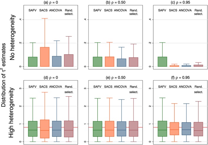
Box plots representing the distribution of τ ² estimates calculated from four combinations of analytical methods (all SAFV, all SACS, all ANCOVA and Rand. select.). Box plots represent select simulation scenarios with θ = 0 and ${\sigma }_{Y_{int}}^2=1$. The horizontal line in the bottom row represents underlying heterogeneity (τ ² = 0.9²). Vertical scales differ for the no (top row) and high (bottom row) heterogeneity plots. Note that outliers are not plotted. SAFV, simple analysis of final values; ANCOVA, analysis of covariance; SACS, simple analysis of change scores; Rand. select., random selection