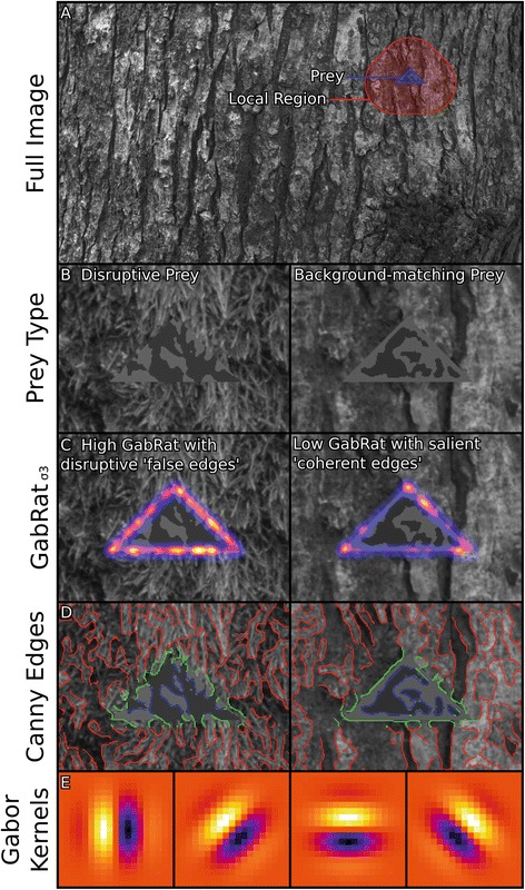
Fig. 1.

Examples of prey and edge disruption measurements. (a) Sample prey highlighted in blue against its background image. The ‘local’ region within a radius of one body-length is highlighted in red. (b) Examples of prey generated with the disruptive algorithm (left) and background-matching algorithm (right). These prey were chosen as their GabRat values were near the upper and lower end of the distribution (see below). (c) Illustration of the GabRat measurement. Red and yellow false colours indicate the perceived edges run orthogonal to the prey’s outline (making disruptive ‘false edges’), blue false colours indicate the perceived edges are parallel to the prey’s outline (making ‘coherent edges’). GabRat values are only measured on outline-pixels, so these values have been smoothed with a Gaussian filter (σ = 3) to illustrate the approximate field of influence. The prey on the left has a high GabRat value of 0.40, while the prey on the right has a low GabRat value (0.20). (d) Canny edges are highlighted in the images. Edges inside the prey are highlighted in blue, edges in the prey’s outline region are green, and edges outside the prey are red. The VisRat and DisRat disruption metrics are formed from the ratios of these edges. (e) Gabor filter kernels (sigma = 3), shown in false colour at the different angles measured