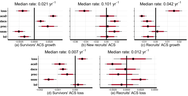
Figure 2. Effect of covariates on the rate at which post-disturbance ACS changes converge to a theoretical steady state (in yr${}^{-1}$).

Covariates are : disturbance intensity ($loss$) , i.e. the proportion of initial ACS loss; mean site’s ACS ($acs0$), and relative forest maturity, i.e. pre-logging plot ACS as a % of $acs0$ ($dacs$); annual precipitation ($prec$); seasonality of precipitation ($seas$), soil bulk density ($bd$). Covariates are centred and standardized. Red and black levels are 80% and 95% credible intervals, respectively. The median rate is the prediction of the convergence rate for an average plot (when all covariates are set to zero). Negative covariate values indicate slowing and positive values indicate accelerating rates. (a) Survivors’ ACS growth. (b) New recruits’ ACS. (c) Recruits’ ACS growth. (d) Survivors’ ACS loss. (e) Recruits’ ACS loss.

DOI: http://dx.doi.org/10.7554/eLife.21394.005

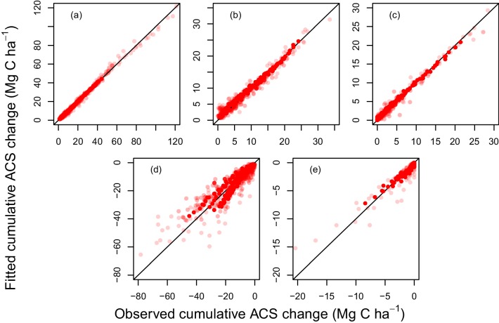
Figure 2—figure supplement 1. Fitted vs observed values of cumulative ACS changes (Mg C ha${}^{-1}$).

(a) Survivors’ cumulative ACS growth. (b) New recruits’ cumulative ACS. (c) Recruits’ cumulative ACS growth; (d) Survivors’ cumulative ACS loss; (e) Recruits’ cumulative ACS loss. The closer the dots are to the x=y line, the better the prediction. Dot transparency is proportional to the observation weight: transparent dots are low-weight observations. Because mortality is a stochastic event, ACS loss has poorer predictions than ACS gain which is a more continuous process.

DOI: http://dx.doi.org/10.7554/eLife.21394.007