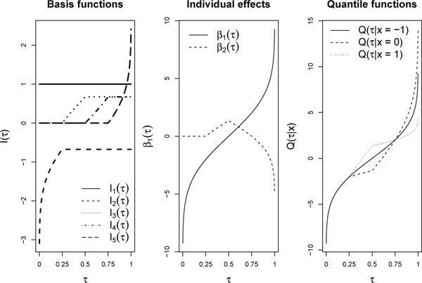
Fig 2.

Plots of the quantile model with M = 5 basis functions with knots at (0.25, 0.5, 0.75) and one covariate x, with θ_.1 = (0, 3, 3, 3, 3) corresponding to basis coefficients for the intercept and θ_.2 = (0, 0, 2, −2, −2) corresponding to basis coefficients for x. The left plot displays the constant basis function (m = 1) and 4 Gaussian basis functions that each correspond to a different quartile of the distribution. The middle plot displays the intercept process β₁(τ), which is the distribution when all covariates are 0, and the covariate effect β₂(τ), defined as the deviation in the intercept process due to a one unit change in x. The final panel displays the conditional quantile function Q(τ|x) = β₁(τ) + xβ₂(τ) for x = −1, x = 0, and x = 1.