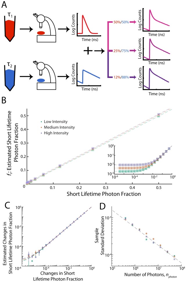
Fig 3. Low-fraction regime.

(A) Samples of dyes with short-lifetime (Erythrosin B) and long-lifetime (Coumarin 153) were prepared, and fluorescence lifetime measurements were collected for each dye separately, leading to separate master photon histograms. Test histograms were constructed by randomly sampling a fixed number of photons, with varying fractions being drawn from the master lists of short-lifetime and long-lifetime photons. These histograms were then analyzed in order to estimate the fraction of short-lifetime photons, f_S. (B) The estimated short-lifetime fraction, f_S, varies linearly with the constructed short-lifetime fraction for three different total photon numbers, with a small offset. Squares: estimate from posterior mode. Dots: estimate from posterior mean. Dashed lines: linear fits with slopes 0.9933 ± 0.0026, 1.0085 ± 0.0024, and 1.0106 ± 0.0031, and offsets of 0.002000 ± 0.0484 × 10⁻⁴, 0.004400 ± 0.0814 × 10⁻⁴, and 0.009500 ± 0.1992 × 10⁻⁴ for low, medium, and high intensities respectively (95% confidence interval). Intensities correspond to data collected at ≈1.5 × 10⁵, 1.2 × 10⁶, and 4.8 × 10⁶ counts per second, for low, medium, and high intensity respectively. Inset: Data from main figure shown on a log-log scale. (C) Changes in the estimated short-lifetime fraction track the known changes in the short-lifetime fraction. Squares: estimate from posterior mode. Dots: estimate from posterior mean. Dashed lines: Linear fits with slopes of 0.9573 ± 0.1895, 1.0013 ± 0.1445, and 0.9580 ± 0.1717, and offsets of (0.2332 ± 0.3712) × 10⁻⁵, (0.3215 ± 0.3088) × 10⁻⁵, and (0.4617 ± 0.4286) × 10⁻⁵ for low, medium, and high intensities respectively (95% confidence interval). (D) Sample standard deviations decrease with increasing photon number as $\approx \sqrt{n_{photon}}$ Squares: Posterior standard deviation Dashed line: power law fit to all intensities with exponent −0.4764 ± 0.0471 (95% confidence interval).