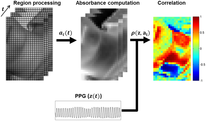
Figure 10. Data processing pipeline.
Each frame was analysed in 0.25 × 0.25 mm regions. Each region’s temporal fluctuations were converted to absorbance using (2). Pearson’s linear correlation coefficient was computed for each waveform using the ground truth PPG waveform, yielding a spatial correlation map showing locations exhibiting strong forward and inverted pulsing. Best viewed in colour.

