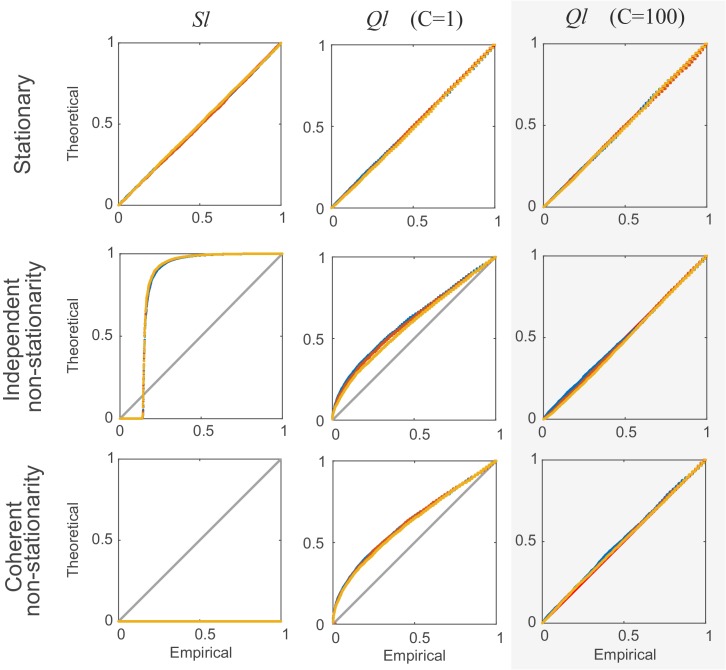
Figure 7. Comparison of non-corrected (${\displaystyle S_{\overline{l}}}$) and stationarity-corrected (${\displaystyle Q_{\overline{l}}}$) pairwise test statistics.

Percentile-percentile plots showing agreement between the theoretical distributions for different test statistics considered in the text (${\displaystyle S_{\overline{l}}}$, ${\displaystyle Q_{\overline{l}}}$ with ${\displaystyle C}$=1, and with ${\displaystyle C}$=100 segments) and the distributions empirically obtained, for the truly stationary case (top row), independent non-stationarity (center row), and non-stationarity coupled among the two units A and B (bottom row). Overlaid are distributions derived from 4000 simulation runs with spike time series analyzed for the three different lags ${\displaystyle l}$= 0 (blue curves), 5 (yellow) and 10 (red). ${\displaystyle \mathrm{\Delta }}$=100 in all cases. Simulations are with non-stationarity implemented as step-type rate-changes (see Materials and methods) with ${\displaystyle m}$=1 and ${\displaystyle L}$=75000. Identity line (bisectrix) is marked in gray. Results for test statistic used for all data analyses in this work highlighted by light-gray box.

DOI: http://dx.doi.org/10.7554/eLife.19428.013

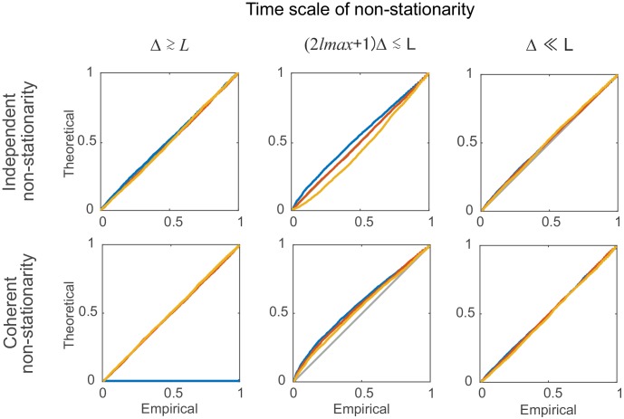
Figure 7—figure supplement 1. Statistical testing under non-stationarity on different time scales: step-like rate change.

Percentile-percentile plots showing agreement between the theoretical and empirical ${\displaystyle Q_{\overline{l}}}$ distributions (computed based on segments of length ${\displaystyle k}$=100 bins, see Supplemental Experimental Procedures). Non-stationarity is implemented here via step-type rate changes with parameters as given in Materials and methods. Overlaid are distributions derived from 4000 simulation experiments with spike time series analyzed for the three different lags ${\displaystyle l}$ = 0 (blue), 5 (red), and 10 (yellow), and ${\displaystyle \mathrm{\Delta }}$=3. Identity line (bisectrix) is marked in gray.

DOI: http://dx.doi.org/10.7554/eLife.19428.014

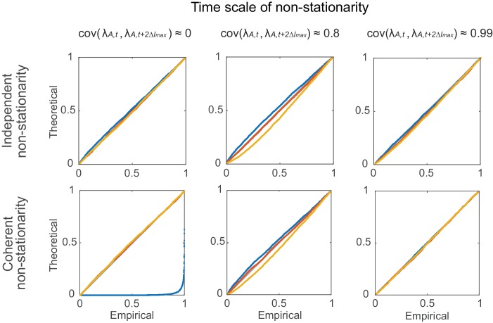
Figure 7—figure supplement 2. Statistical testing under non-stationarity on different time scales: rate covariation.

Agreement in theoretical vs. empirical ${\displaystyle Q_{\overline{l}}}$ (${\displaystyle C}$=100) distributions (P-P-plots as in Figure 7—figure supplement 1) under non-stationary conditions implemented through autoregressive processes (Equations 12–13). Denoting by ${\displaystyle C=\left[dc,cd\right]}$ the coupling matrix of the auto-regressive process, parameters were: ${\displaystyle c}$=0 (top row) and ${\displaystyle d}$=0.4, 0.997, 0.99999 (from left to right); ${\displaystyle d}$=0.4, ${\displaystyle c}$=0.5 (bottom-left), ${\displaystyle d}$=0.995, ${\displaystyle c}$=0.003 (bottom-center), ${\displaystyle d}$=0.9996, ${\displaystyle c}$=0.0004 (bottom-right). Overlaid are distributions derived from 4000 simulation experiments with spike time series analyzed for the three different lags ${\displaystyle l}$ = 0 (blue), 5 (red), and 10 (yellow), and ${\displaystyle \mathrm{\Delta }}$=3. Identity line (bisectrix) is marked in gray.

DOI: http://dx.doi.org/10.7554/eLife.19428.015

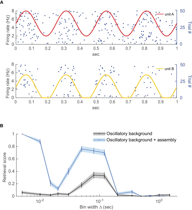
Figure 7—figure supplement 3. Detecting coupling among oscillating units.

Two Poisson units with different mean rates were subjected to a common oscillatory drive. (A) Illustration of the two units’ mean spike rates together with various spike trains drawn from this same process. (B) Detected fraction (from 0 to 1) of significant couplings among the two units as a function of bin width for the case where the units were just driven by the same oscillation but otherwise independent (gray curve) vs. the case where the units exhibited finer-time scale spike interactions on top (blue curve), averaged across n=100 independent runs. For the independent case, coupling is only detected at the time scale of the common oscillation, but not at finer scales. Error bars = SEM.

DOI: http://dx.doi.org/10.7554/eLife.19428.016