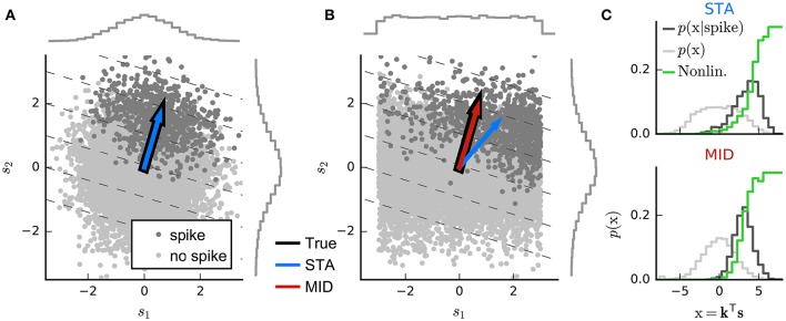
Figure 3.

Geometric illustration of linear filter estimation in the LN model. (A) A two-dimensional stimulus sampled from a Gaussian distribution. Points indicate spike-eliciting (dark gray) and non-spike-eliciting (light gray) stimulus examples with true linear filter shown by the black arrow. For a Gaussian (or more generally, a spherically symmetric) stimulus, the spike-triggered average (STA; blue arrow), given by the mean of all spike-triggered stimuli, recovers the true linear filter. Histograms (insets) show the marginal distributions of stimulus values along each stimulus dimension. Dashed lines indicate “iso-response” hyperplanes (see main text). (B) The same as in (A) except that stimulus dimension s₁ follows a uniform distribution, resulting in a non-spherically symmetric stimulus distribution. The STA no longer points in the same direction as the true linear filter but the maximally informative dimensions (MID; red arrow) estimator is robust to the change in the stimulus distribution. (C) Spike-conditional distribution (p(x|spike)), raw distribution (p(x)) of filtered stimuli, and histogram-based estimates of the spiking nonlinearity (solid green line) for the STA (top) and MID (bottom) for the example in (B). MID seeks the filter that minimizes the overlap between these distributions. The spiking nonlinearity has been rescaled for visualization.