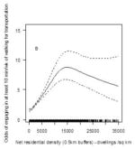
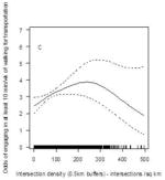
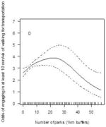
Table 3.
Associations of built environment attributes with any walking for transport (n=11,674)
| Built environment variable (unit) | Buffer size | Model | Linear association | Interactions by study site | Curvilinear (MEV Model) | |
|---|---|---|---|---|---|---|
| OR (95% CI) | p | |||||
| Net residential density (1000 dwellings/km2) | 1km | SEV | 2.33# (1.07, 5.01) | 0.030 | Adelaide Ghent Aarhus Seattle Baltimore |

|
| MEV | 1.90# (0.99, 3.66) | 0.055 | Adelaide Ghent Aarhus Seattle Baltimore |
|||
| 500m | SEV | 1.06# (1.04, 1.07) | <0.001 | NS. | ||
| MEV | 2.51# (1.19, 5.34) | <0.001 | NS. | |||
| Land use mix - 3 uses | 1km | SEV | 2.58 (2.01, 3.30) | <0.001 | Ghent Wellington Seattle |
NONE |
| MEV | 1.52 (1.17, 1.97) | 0.001 | Ghent Wellington Seattle |
|||
| 500m | SEV | 2.22 (1.78, 2.76) | <0.001 | Ghent Seattle |
||
| MEV | 1.48 (1.17, 1.86) | <0.001 | NS. | |||
| Intersection density (100 intersections/km2) | 1km | SEV | 1.71# (1.42, 2.04) | <0.001 | NS. |

|
| MEV | - | - | NS. | |||
| 500m | SEV | 1.43# (1.24, 1.64) | <0.001 | NS. | ||
| MEV | 0.99# (0.79, 1.25) | 0.963 | NS. | |||
| No. parks contained or intersected by buffer (1 park/km2) | 1km | SEV | 1.02 (1.01, 1.03) | 0.005 | NS. |

|
| MEV | 1.00# (0.97, 1.03) | 0.805 | NS. | |||
| 500m | SEV | 1.03 (1.00, 1.06) | 0.026 | Ghent Aarhus Seattle |
||
| MEV | - | - | NS. | |||
Notes. SEV = single-environment-variable model; MEV = multi-environment-variable model; OR = odds ratio; 95 % CI = 95% confidence intervals; ; - = excluded from the model as not a significant independent correlate of the outcome.
significant curvilinear relationship (see corresponding Figure); All regression coefficients are adjusted for respondents’ age, sex, marital status, educational attainment, employment status, administrative-unit socio-economic status, and city.
