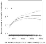
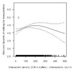
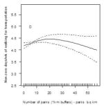
Table 4.
Associations of built environment attributes with days of walking for transportation (n=8,462)
| Built environment variable (unit) | Buffer size | Model | Days/week of walking | Interactions by study site | Curvilinear (MEV Model) | |
|---|---|---|---|---|---|---|
| exp(b) (95% CI) | p | |||||
| Net residential density (1000 dwellings/km2) | 1km | SEV | 1.01# (1.01, 1.01) | <0.001 | NS. |

|
| MEV | 1.09# (1.00, 1.18) | 0.045 | NS. | |||
| 500m | SEV | 1.01# (1.01, 1.01) | <0.001 | NS. | ||
| MEV | 1.10# (1.00, 1.20) | 0.049 | NS. | |||
| Land use mix - 3 uses | 1km | SEV | 1.10 (1.04, 1.17) | 0.002 | NS. | NONE |
| MEV | - | - | ||||
| 500m | SEV | 1.09 (1.03, 1.15) | 0.001 | NS. | ||
| MEV | - | - | ||||
| Intersection density (100 intersections/km2) | 1km | SEV | 1.08 (1.04, 1.12) | <0.001 | Adelaide Ghent Aarhus Wellington Seattle |

|
| MEV | - | - | ||||
| 500m | SEV | 1.04# (1.02, 1.07) | 0.002 | NS. | ||
| MEV | 1.01# (0.96, 1.06) | 0.746 | NS. | |||
| No. parks contained or intersected by buffer (1 park/km2) | 1km | SEV | 1.00# (1.00, 1.01) | 0.018 | Ghent Aarhus North Shore Waitakere Seattle |

|
| MEV | 1.00# (1.00, 1.01) | 0.956 | Ghent Aarhus North Shore Waitakere Seattle |
|||
| 500m | SEV | 1.01 (1.00, 1.01) | 0.018 | NS. | ||
| MEV | - | - | ||||
Notes. SEV = single-environment-variable model; MEV = multi-environment-variable model; exp(b) = antilogarithm of regression coefficient to be interpreted as the proportional increase in the outcome associated with a unit increase in the predictor; exp(95% CI) = antilogarithm of confidence intervals; - = excluded from the model as not a significant independent correlate of the outcome; All regression coefficients are adjusted for respondents’ age, sex, marital status, educational attainment, employment status, administrative-unit socio-economic status, and city.
